TRADERS’ TIPS
May 2026

For this month’s Traders’ Tips, the focus is John F. Ehlers’ article in this issue, “The AutoTune Filter.” Here, we present the May 2026 Traders’ Tips code with possible implementations in various software.
You can right-click on any chart to open it in a new tab or window and view it at it’s originally supplied size, often much larger than the version printed in the magazine.
The Traders’ Tips section is provided to help the reader implement a selected technique from an article in this issue or another recent issue. The entries here are contributed by software developers or programmers for software that is capable of customization.

TradeStation: May 2026
In “The AutoTune Filter” in this issue, John Ehlers presents an adaptive filter that measures dominant market cycles using rolling autocorrelation, then tunes a bandpass filter to produce smoother, more consistent mean-reversion signals with reduced phase distortion. The tuned bandpass output highlights peaks and troughs that can help identify potential market turning points. In the EasyLanguage code, plots 3, 4, and 5 of the charts have been commented out but can be enabled to display additional values, including the minimum autocorrelation used in cycle detection, resulting dominant cycle length, and tuned bandpass output.
Function: $HighPass

{
	$HighPass Function
 	(C) 2004-2024 John F. Ehlers
}

inputs:
	Price(numericseries),
	Period(numericsimple);

variables:
	a1( 0 ),
	b1( 0 ),
	c1( 0 ),
	c2( 0 ),
	c3( 0 );

a1 = ExpValue(-1.414 * 3.14159 / Period);
b1 = 2 * a1 * Cosine(1.414 * 180 / Period);
c2 = b1;
c3 = -a1 * a1;
c1 = (1 + c2 - c3) / 4;

if CurrentBar >= 4 then
 	$HighPass = c1*(Price - 2 * Price[1] + Price[2]) +
	 c2 * $HighPass[1] + c3 * $HighPass[2];
if Currentbar < 4 then
	$HighPass = 0;


Function: $BandPass

{
	Bandpass Function
	(C) 2005 - 2022 John F. Ehlers
}

inputs:
	Price( NumericSeries ),
	Period( NumericSimple ),
	Bandwidth( NumericSimple );

variables:
	G1( 0 ),
	S1( 0 ),
	L1( 0 ),
	BP( 0 );

L1 = Cosine( 360 / Period );
G1 = Cosine( Bandwidth * 360 / Period );
S1 = 1 / G1 - SquareRoot( 1 / (G1 * G1) - 1 );
BP = .5 * (1 - S1) * (Price - Price[2])
 + L1 * (1 + S1) * BP[1] - S1 * BP[2];

if CurrentBar < 3 then
begin
	BP = 0;
end;

$BandPass = BP;

Indicator: AutoTune

{
	TASC MAY 2026
	AutoTune Indicator
	(C) 2025 John F. Ehlers
}

inputs:
	Window( 20 );

variables:
	Filt( 0 ),
	Lag( 0 ),
	J( 0 ),
	Sx( 0 ),
	Sy( 0 ),
	Sxx( 0 ),
	Sxy( 0 ),
	Syy( 0 ),
	X( 0 ),
	Y( 0 ),
	MinCorr( 0 ),
	DC( 0 ),
	BP( 0 );

arrays:
	Corr[100]( 0 );

Filt = $Highpass( Close, Window );
//Cycle test waveform
//Filt = Sine(360*CurrentBar / 20);

//>>>>>>>>> Correlation >>>>>>>>>>>>
for Lag = 1 to Window
begin
	Sx = 0;
	Sy = 0;
	Sxx = 0;
	Sxy = 0;
	Syy = 0;

	for J = 0 to Window - 1
	begin
		X = Filt[J];
		Y = Filt[Lag + J];
		Sx = Sx + X;
		Sy = Sy + Y;
		Sxx = Sxx + X * X;
		Sxy = Sxy + X * Y;
		Syy = Syy + Y * Y;
	end;

	if (Window * Sxx - Sx * Sx > 0) and( Window * Syy -
	Sy * Sy > 0) then Corr[Lag] = (Window * Sxy - Sx * Sy) /
	SquareRoot( (Window * Sxx - Sx * Sx)
	* (Window * Syy - Sy * Sy));
end;

//Find minimum correlation and Dominant Cycle
MinCorr = 1;

for Lag = 1 to Window
begin
	if Corr[Lag] < MinCorr then
	begin
		MinCorr = Corr[Lag];
		DC = 2 * Lag;
	end;
end;

if DC > DC[1] + 2 then
begin
	DC = DC[1] + 2;
end;

if DC < DC[1] - 2 then
begin
	DC = DC[1] - 2;
end;

BP = $Bandpass( Close, DC, .25 );

Plot1( 0, "Zero Line" );
Plot2( Filt, "Filt" );

//Plot3(MinCorr, "", blue, 4, 4);
//Plot4(DC, "", blue, 4, 4);
//Plot5(BP, "", blue, 4, 4);

Strategy: AutoTune Pro Forma

{
AutoTune Pro Forma Strategy
(C) 2025 John F. Ehlers
}
inputs:
	BegDate( 1090101 ),
	EndDate( 1251231 ),
	Window( 26 ),
	BW( .22 ),
	Thresh( -.22 ),
	Delay( 0 );

variables:
	Filt( 0 ),
	Lag( 0 ),
	J( 0 ),
	Sx( 0 ),
	Sy( 0 ),
	Sxx( 0 ),
	Sxy( 0 ),
	Syy( 0 ),
	X( 0 ),
	Y( 0 ),
	MinCorr( 0 ),
	DC( 0 ),
	BP( 0 ),
	ROC( 0 );

arrays:
	Corr[100]( 0 );

Filt = $Highpass( Close, Window );

//>>>>>>>>> Correlation >>>>>>>>>>>>
for Lag = 1 to Window
begin
	Sx = 0;
	Sy = 0;
	Sxx = 0;
	Sxy = 0;
	Syy = 0;

	for J = 0 to Window - 1
	begin
		X = Filt[J];
		Y = Filt[Lag + J];
		Sx = Sx + X;
		Sy = Sy + Y;
		Sxx = Sxx + X * X;
		Sxy = Sxy + X * Y;
		Syy = Syy + Y * Y;
	end;

	if (Window * Sxx - Sx * Sx > 0)
	 and (Window * Syy - Sy * Sy > 0) then
	 	Corr[Lag] = (Window * Sxy - Sx * Sy) /
	 	 SquareRoot( (Window * Sxx - Sx * Sx)
	 	 * (Window * Syy - Sy * Sy) );
end;

//Find minimum correlation and Dominant Cycle
MinCorr = 1;

for Lag = 1 to Window
begin
	if Corr[Lag] < MinCorr then
	begin
		MinCorr = Corr[Lag];
		DC = 2 * Lag;
	end;
end;

if DC > DC[1] + 2 then
begin
	DC = DC[1] + 2;
end;

if DC < DC[1] - 2 then
begin
	DC = DC[1] - 2;
end;

BP = $Bandpass( Close, DC, BW );
ROC = BP - BP[2];

if ROC crosses over 0 and MinCorr < Thresh then
	Buy Next Bar On Open;

if ROC crosses under 0 and MinCorr < Thresh and Filt > 0 then
	Sell Short Next Bar on Open;
A sample chart is shown in Figure 1.

FIGURE 1: TRADESTATION. Demonstrated here is a daily chart of the emini S&P 500 continuous futures contract showing a portion of 2020 with the indicator and strategy applied.
This article is for informational purposes. No type of trading or investment recommendation, advice, or strategy is being made, given, or in any manner provided by TradeStation Securities or its affiliates.
—John Robinson
TradeStation Securities, Inc.
www.TradeStation.com
BACK TO LIST

Wealth-Lab.com: May 2026
WealthLab code is provided here for implementation of the indicator described in John Ehlers’ article in this issue, “The AutoTune Filter.”
The indicator we are providing, named the AutoTune TASC indicator, has two versions: The first gives the output of the autotuned-to-dominant-cycle bandpass filter, but by passing true to the indicator’s optional fourth parameter, you’ll get the min correlation series for use in strategy rules. In our long-only C# version of the pro forma strategy, we normalized the ROC (rate of change) momentum oscillator and decided on a “turn up from under -0.15” as an entry rule.
using WealthLab.TASC;
using WealthLab.Backtest;
using WealthLab.Core;
using WealthLab.Indicators;

namespace WealthScript2026
{
    public class AutoTuneProFormaLong : UserStrategyBase
    {
        public override void Initialize(BarHistory bars)
        {
            _autoTune = AutoTune.Series(bars.Close, 20, 0.2);
            _roc = Momentum.Series(_autoTune, 2) / bars.Close * 100;
            PlotTimeSeriesLine(_roc, "Mo %", "ROC", WLColor.SandyBrown);
            DrawHorzLine(-0.15, WLColor.White, 1, LineStyle.Dashed, "ROC");

            PlotIndicator(_autoTune, WLColor.FromArgb(255, 120, 120, 255), PlotStyle.Line);
            _minCorr = AutoTune.Series(bars.Close, 20, 0.2, true);

            PlotTimeSeriesLine(_minCorr, "MinCorr", "MinCorr", WLColor.White, 2);
            StartIndex = 20;
        }

        public override void Execute(BarHistory bars, int idx)
        {
            if (!HasOpenPosition(bars, PositionType.Long))
            {   // entry
                if (_roc[idx - 1] < -0.15 && _roc.TurnsUp(idx) && _minCorr[idx] < _thresh)
                    PlaceTrade(bars, TransactionType.Buy, OrderType.Market);
            }
            else
            {   // exit
                if (_roc.CrossesUnder(0, idx) && _minCorr[idx] < _thresh)
                    ClosePosition(LastPosition, OrderType.Market);
            }
        }

        IndicatorBase _autoTune;
        IndicatorBase _minCorr;
        TimeSeries _roc;
        double _thresh = 0.22;
    }
}
Figure 2 shows some opportune entry points while avoiding the whipsaws that could have been created by the flat squiggles during February 2025.
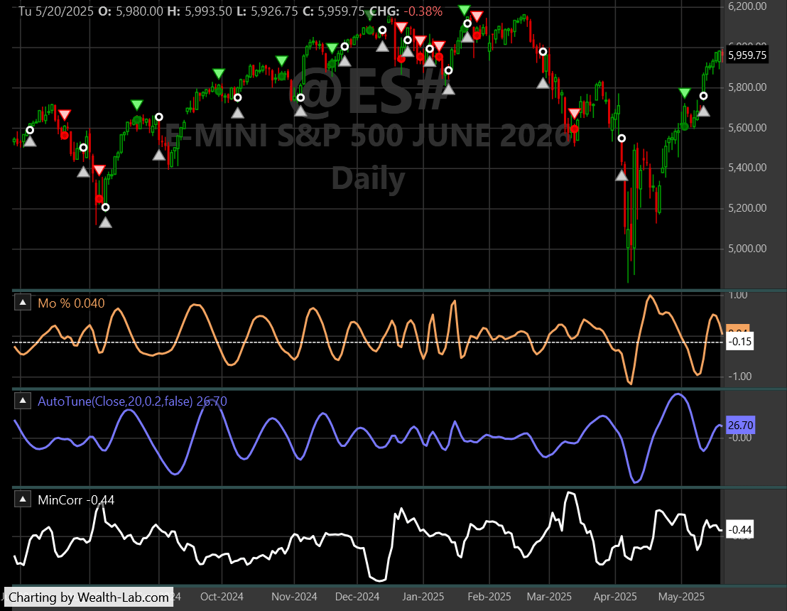
FIGURE 2: WEALTH-LAB. This shows an example of some long trade signals generated by the AutoTune indicator.
—Robert Sucher
Wealth-Lab team
www.wealth-lab.com
BACK TO LIST

NinjaTrader: May 2026
In “The AutoTune Filter” in this issue, John Ehlers presents an indicator he named the AutoTune indicator. An indicator based on the description given in the article is available for download at the following link for NinjaTrader 8:
Once the file is downloaded, you can import the indicator into NinjaTrader 8 from within the control center by selecting Tools → Import → NinjaScript Add-On and then selecting the downloaded file for NinjaTrader 8.
You can review the indicator source code in NinjaTrader 8 by selecting the menu New → NinjaScript Editor → Indicators folder from within the control center window and selecting the file.
A sample chart is shown in Figure 3.
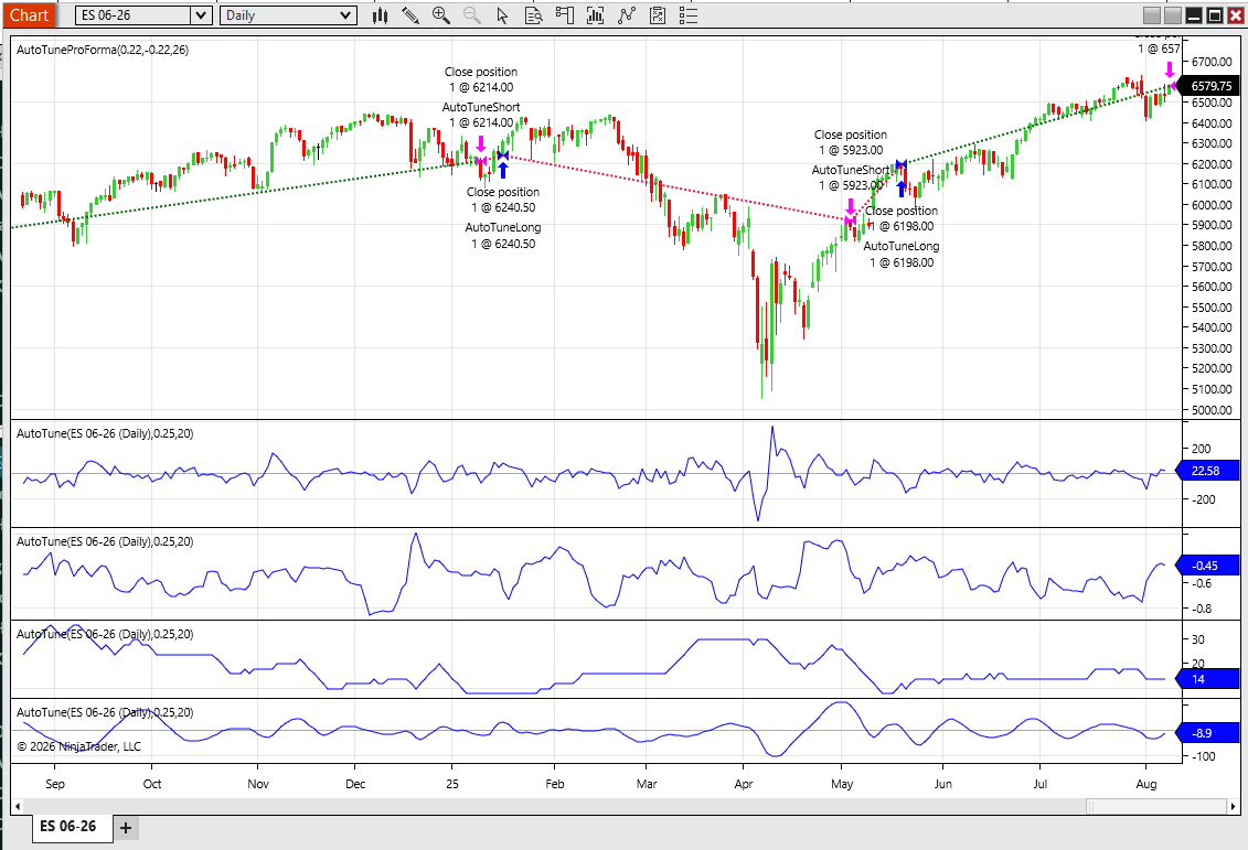
FIGURE 3: NINJATRADER. The AutoTune indicator is demonstrated on a daily chart of emini S&P 500 futures (ES).
NinjaScript uses compiled DLLs that run native, not interpreted, to provide you with the highest performance possible.
—Eduard
NinjaTrader, LLC
www.ninjatrader.com
BACK TO LIST

RealTest: May 2026
Provided here is coding for use in the RealTest platform to implement the AutoTune indicator described in John Ehlers’ article in this issue, “The AutoTune Filter.”
Notes:
	John Ehlers "The AutoTune Filter", TASC May 2026.
	Implements the AutoTune Filter indicator and pro forma strategy.
	Rolling autocorrelation of highpass-filtered data identifies
	the dominant cycle period, which dynamically tunes a bandpass
	filter for mean-reversion signals.
	The Highpass and Bandpass filter functions from previous Ehlers
	articles are implemented inline in the Data section.

Import:
	DataSource:	Norgate
	IncludeList:	&ES_CCB
	StartDate:	2008-01-01
	EndDate:	Latest
	SaveAs:	es.rtd

Settings:
	DataFile:	es.rtd
	BarSize:	Daily
	StartDate:	2009-01-01
	EndDate:	Latest

Parameters:
	Window:	20
	BW:	0.25
	Thresh:	-0.3

Data:
	// Common constants for Ehlers filters
	decay_factor:	-1.414 * 3.14159
	phase_angle:	1.414 * 180

	// Highpass Filter of Close at Window period
	hp_a1:	exp(decay_factor / Window)
	hp_b1:	2 * hp_a1 * Cosine(phase_angle / Window)
	hp_c2:	hp_b1
	hp_c3:	-hp_a1 * hp_a1
	hp_c1:	(1 + hp_c2 - hp_c3) / 4
	Filt:	if(BarNum >= 4, hp_c1 * (Close - 2 * Close[1] + Close[2]) + hp_c2 * Filt[1] + hp_c3 * Filt[2], 0)

	// Rolling autocorrelation at lags 1 through 20 (must match Window)
	Corr1:	Correl(Filt, Filt[1], Window)
	Corr2:	Correl(Filt, Filt[2], Window)
	Corr3:	Correl(Filt, Filt[3], Window)
	Corr4:	Correl(Filt, Filt[4], Window)
	Corr5:	Correl(Filt, Filt[5], Window)
	Corr6:	Correl(Filt, Filt[6], Window)
	Corr7:	Correl(Filt, Filt[7], Window)
	Corr8:	Correl(Filt, Filt[8], Window)
	Corr9:	Correl(Filt, Filt[9], Window)
	Corr10:	Correl(Filt, Filt[10], Window)
	Corr11:	Correl(Filt, Filt[11], Window)
	Corr12:	Correl(Filt, Filt[12], Window)
	Corr13:	Correl(Filt, Filt[13], Window)
	Corr14:	Correl(Filt, Filt[14], Window)
	Corr15:	Correl(Filt, Filt[15], Window)
	Corr16:	Correl(Filt, Filt[16], Window)
	Corr17:	Correl(Filt, Filt[17], Window)
	Corr18:	Correl(Filt, Filt[18], Window)
	Corr19:	Correl(Filt, Filt[19], Window)
	Corr20:	Correl(Filt, Filt[20], Window)

	// Minimum correlation across all lags
	MinCorr:	Min(Corr1, Corr2, Corr3, Corr4, Corr5, Corr6, Corr7, Corr8, Corr9, Corr10, Corr11, Corr12, Corr13, Corr14, Corr15, Corr16, Corr17, Corr18, Corr19, Corr20)

	// Lag at which minimum correlation occurs => dominant half-cycle
	DClag:	Switch(MinCorr, Corr1, 1, Corr2, 2, Corr3, 3, Corr4, 4, Corr5, 5, Corr6, 6, Corr7, 7, Corr8, 8, Corr9, 9, Corr10, 10, Corr11, 11, Corr12, 12, Corr13, 13, Corr14, 14, Corr15, 15, Corr16, 16, Corr17, 17, Corr18, 18, Corr19, 19, Corr20, 20)

	// Dominant Cycle period, clamped to change no more than 2 per bar
	rawDC:	2 * DClag
	DC:	Bound(rawDC, nonan(DC[1], rawDC) - 2, nonan(DC[1], rawDC) + 2)

	// Bandpass Filter of Close tuned to dominant cycle
	bp_L1:	Cosine(360 / DC)
	bp_G1:	Cosine(BW * 360 / DC)
	bp_S1:	1 / bp_G1 - Sqr(1 / (bp_G1 * bp_G1) - 1)
	BP:	if(BarNum >= 4 and not IsNaN(DC), 0.5 * (1 - bp_S1) * (Close - Close[2]) + bp_L1 * (1 + bp_S1) * nonan(BP[1]) - bp_S1 * nonan(BP[2]), 0)

	// Rate of change (two-bar difference for smoother response)
	bpROC:	BP - BP[2]

	// Trading signals
	goLong:	Cross(bpROC, 0) and MinCorr < Thresh
	goShort:	Cross(0, bpROC) and MinCorr < Thresh and Filt > 0

Charts:
	BP:	BP {|}
	Zero:	0 {|}
//	Filt:	Filt {|}
//	MinCorr:	MinCorr {|}
//	DC:	DC {|}

Strategy: AT_Long
	Side:	Long
	Quantity:	1
	EntrySetup:	goLong
	ExitRule:	goShort

Strategy: AT_Short
	Side:	Short
	Quantity:	1
	EntrySetup:	goShort
	ExitRule:	goLong
—Marsten Parker
MHP Trading
mhp@mhptrading.com
BACK TO LIST

TradingView: May 2026
The TradingView Pine Script code presented here implements the AutoTune Filter as presented by John Ehlers in his article in this issue, “The AutoTune Filter.”
//  TASC Issue: May 2026
//     Article: A Rolling Autocorrelation Function
//              The AutoTune Filter
//  Article By: John F. Ehlers
//    Language: TradingView's Pine Script® v6
// Provided By: PineCoders, for tradingview.com

//@version=6
indicator("TASC 2026.05 The AutoTune Filter", "AutoTune")

//#region Inputs

enum disp
    F = "Filter"
    M = "Min. Correlation"
    D = "Dominant Cycle"
    B = "Band Pass"

src = input.source(close, "Source:")
window = input.int(20, "Window:")
dispType = input.enum(disp.F, title = "Output:")

//#endregion

//#region Functions

// @function High Pass Filter.
HP(float _src, int _period) =>

    float Q = math.exp(-1.414*math.pi/_period)
    float c1 = 2.0*Q*math.cos(1.414*math.pi/_period)
    float c2 = Q*Q
    float a0 = (1 + c1 + c2)/4
    float hp = 0.0
    if bar_index >= 4
        hp := a0*(_src - 2*_src[1] +
              _src[2]) + c1*hp[1] - c2*hp[2]
    hp

// @function Bandpass
BP(float _src = close,
   int _period = 20,
   float _bandwidth=0.25) =>

    float L1 = math.cos(2.0*math.pi/_period)
    float G1 = math.cos(_bandwidth*2.0*math.pi/_period)
    float S1 = 1.0/G1 - math.sqrt(1.0/(G1*G1) - 1.0)
    float BP = 0.0

    BP := 0.5*(1.0 - S1)*(_src - _src[2]) +
     L1*(1.0 + S1)*nz(BP[1]) - S1*nz(BP[2])

    if bar_index < 3
        BP := 0.0
    BP

// @function AutoTune Filter.
AF(float _src = close,
   int _window = 20,
   float _bandwidth=0.25) =>

    array<float> Corr = array.new<float>(100)
    float Filt = HP(_src, _window)
    // Correlation
    for lag = 1 to _window
        float Sx = 0.0
        float Sy = 0.0
        float Sxx = 0.0
        float Sxy = 0.0
        float Syy = 0.0
        for J = 0 to _window - 1
            float X = Filt[J]
            float Y = Filt[lag + J]
            Sx += X
            Sy += Y
            Sxx += X*X
            Sxy += X*Y
            Syy += Y*Y
        if ((_window*Sxx - Sx*Sx) > 0.0) and
         ((_window*Syy - Sy*Sy) > 0.0)

            Corr.set(lag,
            (_window*Syy - Sy*Sy)/math.sqrt(
             (_window*Sxx - Sx*Sx)*(_window*Syy - Sy*Sy)))

    float MinCorr = 1.0
    int DC = 0
    for lag = 1 to _window
        if Corr.get(lag) < MinCorr
            MinCorr := Corr.get(lag)
            DC := 2*lag
    if DC > DC[1] + 2
        DC := DC[1] + 2
    if DC < DC[1] - 2
        DC := DC[1] - 2

    float BP = BP(_src, DC, _bandwidth)
    [Filt, MinCorr, DC, BP]

//#endregion

//#region Calc

[f, mc, dc, bp] = AF(src, window)

//#endregion

//#region Display

float show_disp = switch
    dispType == disp.F => f
    dispType == disp.M => mc
    dispType == disp.D => dc
    dispType == disp.B => bp

hline(0, title = "Zero")
plot(show_disp, title = "Display")

//#endregion
The indicator is available on TradingView from the PineCodersTASC account at https://www.tradingview.com/u/PineCodersTASC/#published-scripts.
An example chart is shown in Figure 4.
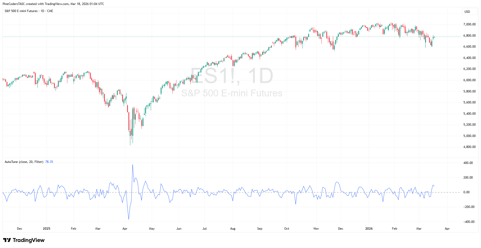
FIGURE 4: TRADINGVIEW. An example of John Ehlers’ AutoTune indicator is plotted beneath a daily chart of emini S&P 500 futures (ES).
—PineCoders, for TradingView
www.TradingView.com
BACK TO LIST

Neuroshell Trader: May 2026
The indicator and demonstration strategy presented in John Ehlers’ article in this issue, “The AutoTune Filter,” can be easily implemented in NeuroShell Trader using NeuroShell Trader’s ability to call external dynamic linked libraries. Dynamic linked libraries can be written in C, C++, or Power Basic.
After moving the code given in the article to your preferred compiler and creating a DLL, you can insert the resulting indicator(s) as follows:
- Select “New indicator...” from the insert menu.
- Choose the “External program & library calls” category.
- Select the appropriate external DLL call indicator.
- Set up the parameters to match your DLL.
- Select the finished button.
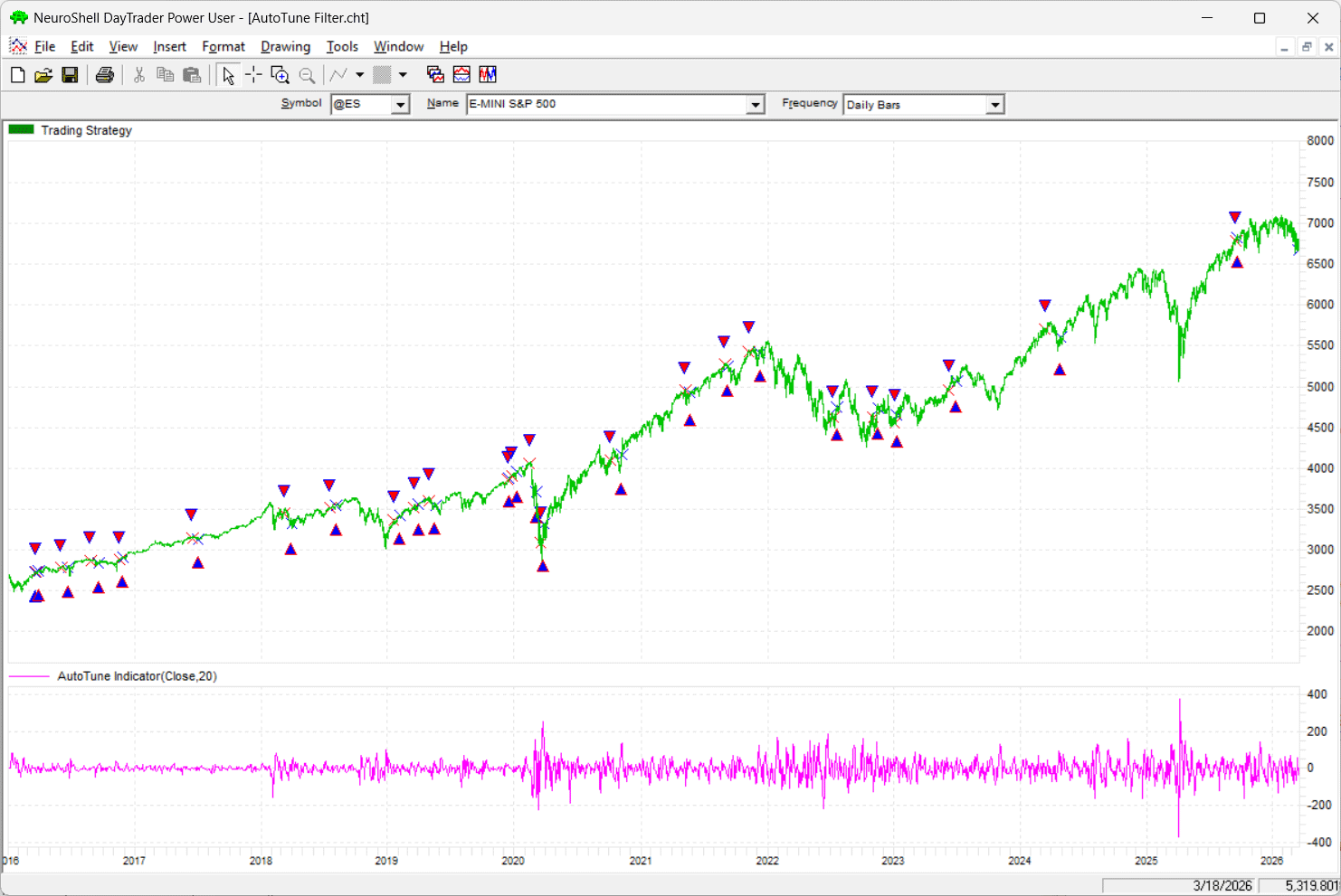
FIGURE 5: NEUROSHELL TRADER. This NeuroShell Trader chart of emini S&P 500 futures (ES) shows the AutoTune indicator and the example trading strategy based on the indicator.
Users of NeuroShell Trader can go to the Stocks & Commodities section of the NeuroShell Trader free technical support website to download a copy of this or any previous Traders’ Tips.
—Ward Systems Group, Inc.
sales@wardsystems.com
www.neuroshell.com
BACK TO LIST

The Zorro Project: May 2026
Any price curve is a mix of many long-term and short-term cycles. But once in a while, a dominant market cycle emerges and can be exploited for trading. In his article in this issue, “The AutoTune Filter,” John Ehlers describes an algorithm for detecting such dominant cycles and using them to tune a bandpass filter. The EasyLanguage code given in the article can be directly converted to C for Zorro. In fact, ChatGPT does it in a few seconds. First, here is the cycle detector:
var MinCorr, Filt;
var AutoTune(vars Data,int Window)
{
	Filt = HighPass3(Data,Window);
	vars HP = series(Filt);
	var Corr[256];
	int Lag, J;

	for(Lag = 1; Lag <= Window; Lag++)
	{
		var Sx = 0., Sy = 0.;
		var Sxx = 0., Sxy = 0., Syy = 0.;

		for(J = 0; J < Window; J++)
		{
			var X = HP[J];
			var Y = HP[Lag + J];
			Sx  += X; Sy  += Y;
			Sxx += X*X; Sxy += X*Y; Syy += Y*Y;
		}

		var Den1 = Window*Sxx - Sx*Sx;
		var Den2 = Window*Syy - Sy*Sy;

		if(Den1 > 0. && Den2 > 0.)
			Corr[Lag] = (Window*Sxy - Sx*Sy) / sqrt(Den1*Den2);
		else
			Corr[Lag] = 0.;
	}

	MinCorr = 1.;
	var DC = Window;

	for(Lag = 1; Lag <= Window; Lag++)
		if(Corr[Lag] < MinCorr) {
			MinCorr = Corr[Lag];
			DC = 2*Lag;
		}

	vars DCs = series(DC,2);
	return DCs[0] = clamp(DC,DCs[1]-2.,DCs[1]+2.);
}
The output is then used for the center frequency of a bandpass filter. Since Zorro has already a bandpass filter in its arsenal, I named it “BandPass2”:
var BandPass2(vars Data, int Period, var Bandwidth)
{
	var L1 = cos(2.*PI/Period);
	var G1 = cos(Bandwidth*2.*PI/Period);
	var S1 = 1./G1 - sqrt(1./(G1*G1) - 1.);
	vars BP = series(0,3);
	return BP[0] = 0.5*(1.-S1)*(Data[0]-Data[2])
		      + L1*(1.+S1)*BP[1] - S1*BP[2];
}
Here is the code for reproducing Ehlers’ ES chart in the article:
function run()
{
	BarPeriod = 1440;
	StartDate = 2024;
	EndDate = 2025;
	asset("ES");

	var DC = AutoTune(seriesC(),20);
	var BP = BandPass2(seriesC(),DC,0.25);
	plot("Zero",0,NEW,BLACK);
	plot("BP",BP,LINE,BLUE);
}
The resulting chart is shown in Figure 6.
FIGURE 6: ZORRO. The AutoTune filter is demonstrated on a chart of emini S&P 500 futures (ES).
The tiny differences to Ehlers’ chart are caused by generating a continuous curve from ES futures contracts, which depends on the most recent contract.
Next, we will use the bandpass output for a trading signal. We will use walk-forward analysis, not in-sample optimization, to produce realistic results here in our test. We will set up the strategy to reinvest profits using the square root rule. The code to do this is as follows:
function run()
{
	BarPeriod = 1440;
	StartDate = 2010;
	EndDate = 2025;
	Capital = 100000;
	asset("ES");

	set(TESTNOW,PARAMETERS);
	NumWFOCycles = 10;
	int Window = optimize("Window",26,10,30,2);
	var BW = optimize("BW",0.22,0.10,0.30,0.01);
	var Thresh = -optimize("Thresh",0.22,0.1,0.3,0.01);

	var DC = AutoTune(seriesC(),Window);
	var BP = BandPass2(seriesC(),DC,BW);
	vars ROCs = series(BP-ref(BP,2));

	Lots = 0.5*(Capital+sqrt(1.+ProfitTotal/Capital))/MarginCost;
	MaxLong = MaxShort = 1;
	if(crossOver(ROCs,0) && MinCorr < Thresh)
		enterLong();
	if(crossUnder(ROCs,0) && MinCorr < Thresh && Filt > 0)
		enterShort();
}
Training and testing produces the realistic equity curve shown in Figure 7. This curve does not look as impressive as the sample equity curve shown in Ehlers’ article based on the pro-forma strategy, but the CAGR is in the 25% area, which is a much better performance than a buy-and-hold strategy.
FIGURE 7: ZORRO. Shown here is the equity curve after testing a trading strategy based on the AutoTune filter.
The code can be downloaded from the 2026 script repository on https://financial-hacker.com. The Zorro platform can be downloaded from https://zorro-project.com.
—Petra Volkova
The Zorro Project by oP group Germany
https://zorro-project.com
BACK TO LIST
Python: May 2026
Provided here is Python code to implement concepts described in John Ehlers’ article in this issue, “The AutoTune Filter.”
Readers will also find the following code in a Jupyter notebook on GitHub at: https://github.com/jainraje/TraderTipArticles.
"""

Python code to implement concepts in Technical Analysis of Stocks & Commodiities magazine
May 2026 article "The AutoTune Filter" by John F Ehlers. This python code is provided
for TraderTips section of the magazine.

Written By:
Rajeev Jain, Mar 2026
jainraje@yahoo,com

All code available in GitHub:
https://github.com/jainraje/TraderTipArticles/

"""


# import required python libraries
import pandas as pd
import numpy as np
import matplotlib.pyplot as plt
import yfinance as yf
import math

print(yf.__version__)


# HELPER FUNCTIONS
def highpass_filter(price, period):
    price = np.asarray(price, dtype=float)
    n = len(price)
    hp = np.zeros(n, dtype=float)

    Q  = math.exp(-1.414 * math.pi / period)
    c1 = 2 * Q * math.cos(1.414 * math.pi / period)
    c2 = Q * Q
    a0 = (1 + c1 + c2) / 4.0

    for t in range(2, n):
        hp[t] = (
            a0 * (price[t] - 2 * price[t-1] + price[t-2]) +
            c1 * hp[t-1] -
            c2 * hp[t-2]
        )
    return hp


def bandpass_single_step(close, bp_prev1, bp_prev2, period, bandwidth):

    if period <= 0:
        return 0.0

    L1 = math.cos(2 * math.pi / period)
    G1 = math.cos(bandwidth * 2 * math.pi / period)
    S1 = 1.0 / G1 - math.sqrt(1.0 / (G1 * G1) - 1.0)

    return (
        0.5 * (1.0 - S1) * (close[0] - close[2]) +
        L1 * (1.0 + S1) * bp_prev1 -
        S1 * bp_prev2
    )

# Retrieve price data via Yahoo Finance

symbol = '^GSPC'
symbol = 'ES=F'
ohlcv = yf.download(
    symbol,
    start="2000-01-01",
    end="2026-03-18",
    group_by="Ticker",
    auto_adjust=True,
    progress=False,
)
ohlcv = ohlcv.stack('Ticker', future_stack=True).reset_index().set_index('Date')
ohlcv


# inspect closing price line plot
ax = ohlcv['Close'].plot(grid=True, title=f'Ticker={symbol}')


# AutoTune Indicator and AutoTune Plot functions

def autotune_indicator(close, window=20, bp_bandwidth=0.25):

    close = np.asarray(close, dtype=float)
    n = len(close)

    filt = highpass_filter(close, window)
    mincorr = np.ones(n, dtype=float)
    dc = np.zeros(n, dtype=float)
    bp = np.zeros(n, dtype=float)

    for t in range(window, n):
        # correlation window: last `window` filt values ending at t
        x = filt[t-window+1 : t+1]  # length = window

        # For each lag = 1..window, compute correlation with lagged version
        best_corr = 1.0
        best_lag = 1

        for lag in range(1, window + 1):
            # y is x shifted back by `lag` bars in the underlying filt series
            idx_start = t - window + 1 - lag
            idx_end   = t + 1 - lag

            if idx_start < 0:
                continue

            y = filt[idx_start:idx_end]
            if len(y) != window:
                continue

            Sx = x.sum()
            Sy = y.sum()
            Sxx = np.dot(x, x)
            Syy = np.dot(y, y)
            Sxy = np.dot(x, y)

            denom_x = window * Sxx - Sx * Sx
            denom_y = window * Syy - Sy * Sy
            if denom_x <= 0 or denom_y <= 0:
                continue

            corr = (window * Sxy - Sx * Sy) / math.sqrt(denom_x * denom_y)
            if corr < best_corr:
                best_corr = corr
                best_lag = lag

        # Dominant cycle
        local_dc = 2.0 * best_lag
        if t > 0:
            if local_dc > dc[t-1] + 2:
                local_dc = dc[t-1] + 2
            if local_dc < dc[t-1] - 2:
                local_dc = dc[t-1] - 2

        mincorr[t] = best_corr
        dc[t] = local_dc

        # Bandpass at this bar (needs t >= 2)
        if t >= 2 and dc[t] > 0:
            bp[t] = bandpass_single_step(
                close[t-2:t+1], bp[t-1], bp[t-2], dc[t], bp_bandwidth
            )

    return filt, mincorr, dc, bp


def plot_autotune_filter(df):

    import matplotlib.pyplot as plt

    fig, (ax1, ax2) = plt.subplots(
        2, 1, figsize=(9,6), sharex=True,
        gridspec_kw={"height_ratios": [2, 1]}
    )

    # Overall title
    fig.suptitle(f"Ticker={symbol}", fontsize=14)

    # Top: Close in black
    ax1.plot(df.index, df["Close"], color="black", label="Close")
    ax1.set_title("Close")
    ax1.legend(loc="upper left")
    ax1.grid(True)

    # Bottom: Filt in dark blue
    ax2.plot(df.index, df["Filt"], color="darkblue", label="ATF")
    ax2.axhline(y=0, color="black", linewidth=1)  # horizontal line at zero
    ax2.set_title("AutoTune Filter Indicator")
    ax2.legend(loc="upper left")
    ax2.grid(True)

    plt.tight_layout()
    plt.show()


# Run the indicator function and plot results
# using slicing techniques to plot last 126 days (aka 6M)

df = ohlcv.copy()
df["Filt"], df["MinCorr"], df["DC"], df["BP"] = autotune_indicator(df['Close'], window=20, bp_bandwidth=0.25)
df


plot_autotune_filter(df[-126:])
An example plot of the AutoTune indicator is shown in Figure 8.
Figure 8: PYTHON. An example plot of John Ehlers’ AutoTune indicator is demonstrated on a chart of emini S&P 500 futures (ES).
—Rajeev Jain
jainraje@yahoo.com
BACK TO LIST
Originally published in the May 2026 issue of
Technical Analysis of STOCKS & COMMODITIES magazine.
All rights reserved. © Copyright 2026, Technical Analysis, Inc.