TRADERS’ TIPS
June 2025

For this month’s Traders’ Tips, the focus is John F. Ehlers’ article in this issue, “Making A Better Oscillator.” Here, we present the June 2025 Traders’ Tips code with possible implementations in various software.
You can right-click on any chart to open it in a new tab or window and view it at it’s originally supplied size, often much larger than the version printed in the magazine.
The Traders’ Tips section is provided to help the reader implement a selected technique from an article in this issue or another recent issue. The entries here are contributed by software developers or programmers for software that is capable of customization.

TradeStation: June 2025
In the article “Making A Better Oscillator” in this issue, John Ehlers introduces a new indicator he calls the cybernetic oscillator. This indicator applies a multistep filter. The data is smoothed using a highpass filter ($HighPass function), which is then smoothed using the lowpass filter ($SuperSmoother function). The result is then scaled to its RMS (root mean squared).
Function: Cybernetic Oscillator
{
	TASC JUN 2025
	Cybernetic Oscillator
	(C) 2025 John F. Ehlers
}

inputs:
	HPLength( 30 ),
	LPLength( 20 );

variables:
	HP( 0 ),
	LP( 0 ),
	RMS( 0 ),
	CyberneticOsc( 0 );

HP = $HighPass(Close, HPLength);
LP = $SuperSmoother(HP, LPLength);
RMS = $RMS(LP, 100);

if RMS <> 0 then
	CyberneticOsc = LP / RMS;

Plot1( CyberneticOsc, "Cybernetic Osc" );
Plot2( 0, "Zero Line" );

Function: $HighPass
{
	$HighPass Function
 	(C) 2004-2025 John F. Ehlers
}

inputs:
	Price(numericseries),
	Period(numericsimple);

variables:
	a1( 0 ),
	b1( 0 ),
	c1( 0 ),
	c2( 0 ),
	c3( 0 );

a1 = ExpValue(-1.414 * 3.14159 / Period);
b1 = 2 * a1 * Cosine(1.414 * 180 / Period);
c2 = b1;
c3 = -a1 * a1;
c1 = (1 + c2 - c3) / 4;

if CurrentBar >= 4 then
 	$HighPass = c1*(Price - 2 * Price[1] + Price[2]) +
	 c2 * $HighPass[1] + c3 * $HighPass[2];
if Currentbar < 4 then
	$HighPass = 0;

Function: $SuperSmoother
{
	$SuperSmoother Function
 	(C) 2004-2025 John F. Ehlers
}

inputs:
	Price(numericseries),
	Period(numericsimple);

variables:
	a1( 0 ),
	b1( 0 ),
	c1( 0 ),
	c2( 0 ),
	c3( 0 );

a1 = ExpValue(-1.414 * 3.14159 / Period);
b1 = 2 * a1 * Cosine(1.414 * 180 / Period);
c2 = b1;
c3 = -a1 * a1;
c1 = 1 - c2 - c3;

if CurrentBar >= 4 then
	$SuperSmoother = c1*(Price + Price[1]) / 2
	 + c2 * $SuperSmoother[1] + c3 * $SuperSmoother[2];
if CurrentBar < 4 then
	$SuperSmoother = Price;

Indicator: $RMS
{
	RMS Function
	(C) 2015-2025 John F. Ehlers
}

inputs:
	Price( numericseries ),
	Length( numericsimple );

variables:
	SumSq( 0 ),
	count( 0 );

SumSq = 0;

for count = 0 to Length - 1
begin
	SumSq = SumSq + Price[count] * Price[count];
end;

If SumSq <> 0 then
	$RMS = SquareRoot(SumSq / Length);
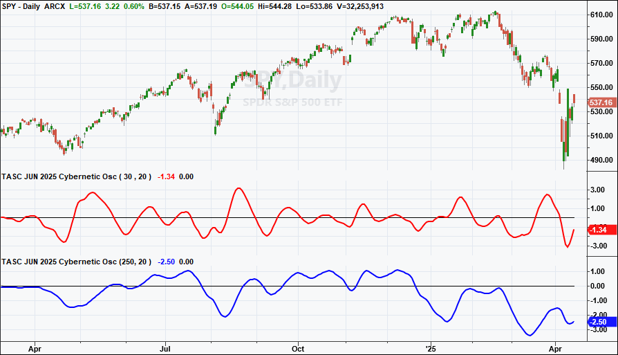
A sample chart is shown in Figure 1.

FIGURE 1: TRADESTATION. This is a daily chart of SPY showing a portion of 2024 and 2025 with indicator applied twice.
This article is for informational purposes. No type of trading or investment recommendation, advice, or strategy is being made, given, or in any manner provided by TradeStation Securities or its affiliates.
—John Robinson
TradeStation Securities, Inc.
www.TradeStation.com
BACK TO LIST

MetaStock: June 2025
John Ehlers’ article in this issue, “Making A Better Oscillator,” introduces his indicator he calls the cybernetic oscillator and also offers an example simple rate-of-change trading strategy to demonstrate using the oscillator in a strategy. Here are the formulas to add that indicator and system test to MetaStock:
The Cybernetic Oscillator:

{by John Ehlers}
HPLen:= 30;
LPLen:= 20;

{High Pass filter of Close}
a1:= exp(-1.414*3.14159 / HPLen);
b1:= 2*a1*Cos(1.414*180 / HPLen);
c1:= -a1*a1;
x1:= (1 + b1 - c1) / 4;
HP1:= x1*(C - Ref(2*C,-1) + Ref(C, -2)) + b1*Prev + c1*Ref(Prev, -1);

{Super Smoother of High Pass}
a2:= exp(-1.414*3.14159 / LPLen);
b2:= 2*a2*Cos(1.414*180 / LPLen);
c2:= -a2*a2;
x2:= (1 + b2 - c2) / 4;
LP1:= x2*(Sum(HP1,2)/2) + b2*Prev + c2*Ref(Prev, -1);

{Root Mean Square of Super Smoother}
RMS:= SQRT(Sum(LP1 * LP1, 100) / 100);

{divide by zero trap}
denom:= if(RMS = 0, -1, RMS);
If(denom = -1, 0, LP1/denom)

Simpel Rate of Change Strategy

Buy Order:
LPLen:= 20;
fastHPLen:= 55;
slowHPLen:= 156;

{Super Smoother of Close}
a1:= exp(-1.414*3.14159 / LPLen);
b1:= 2*a1*Cos(1.414*180 / LPLen);
c1:= -a1*a1;
x1:= (1 + b1 - c1) / 4;
LP1:= x1*(Sum(C,2)/2) + b1*Prev + c1*Ref(Prev, -1);

{fast High Pass filter of Super Smoother}
a2:= exp(-1.414*3.14159 / fastHPLen);
b2:= 2*a2*Cos(1.414*180 / fastHPLen);
c2:= -a2*a2;
x2:= (1 + b2 - c2) / 4;
HP1:= x2*(LP1 - Ref(2*LP1,-1) + Ref(LP1, -2)) + b2*Prev + c2*Ref(Prev, -1);
ROC1:= HP1 - Ref(HP1, -2);

{slow High Pass filter of Super Smoother}
a3:= exp(-1.414*3.14159 / slowHPLen);
b3:= 2*a3*Cos(1.414*180 / slowHPLen);
c3:= -a3*a3;
x3:= (1 + b3 - c3) / 4;
HP2:= x3*(LP1 - Ref(2*LP1,-1) + Ref(LP1, -2)) + b3*Prev + c3*Ref(Prev, -1);
ROC2:= HP2 - Ref(HP2, -2);

ROC1>0 AND ROC2>0


Sell Order:
LPLen:= 20;
fastHPLen:= 55;
slowHPLen:= 156;

{Super Smoother of Close}
a1:= exp(-1.414*3.14159 / LPLen);
b1:= 2*a1*Cos(1.414*180 / LPLen);
c1:= -a1*a1;
x1:= (1 + b1 - c1) / 4;
LP1:= x1*(Sum(C,2)/2) + b1*Prev + c1*Ref(Prev, -1);

{fast High Pass filter of Super Smoother}
a2:= exp(-1.414*3.14159 / fastHPLen);
b2:= 2*a2*Cos(1.414*180 / fastHPLen);
c2:= -a2*a2;
x2:= (1 + b2 - c2) / 4;
HP1:= x2*(LP1 - Ref(2*LP1,-1) + Ref(LP1, -2)) + b2*Prev + c2*Ref(Prev, -1);
ROC1:= HP1 - Ref(HP1, -2);

{slow High Pass filter of Super Smoother}
a3:= exp(-1.414*3.14159 / slowHPLen);
b3:= 2*a3*Cos(1.414*180 / slowHPLen);
c3:= -a3*a3;
x3:= (1 + b3 - c3) / 4;
HP2:= x3*(LP1 - Ref(2*LP1,-1) + Ref(LP1, -2)) + b3*Prev + c3*Ref(Prev, -1);
ROC2:= HP2 - Ref(HP2, -2);

ROC1<0 AND ROC2<0
—William Golson
MetaStock Technical Support
MetaStock.com
BACK TO LIST

Wealth-Lab.com: June 2025
In his article in this issue titled “Making A Better Oscillator,” John Ehlers introduces his cybernetic oscillator. We are offering this new oscillator in WealthLab’s TASC indicator library (named CyberneticOsc), so the user can drag and drop it into charts or strategies.
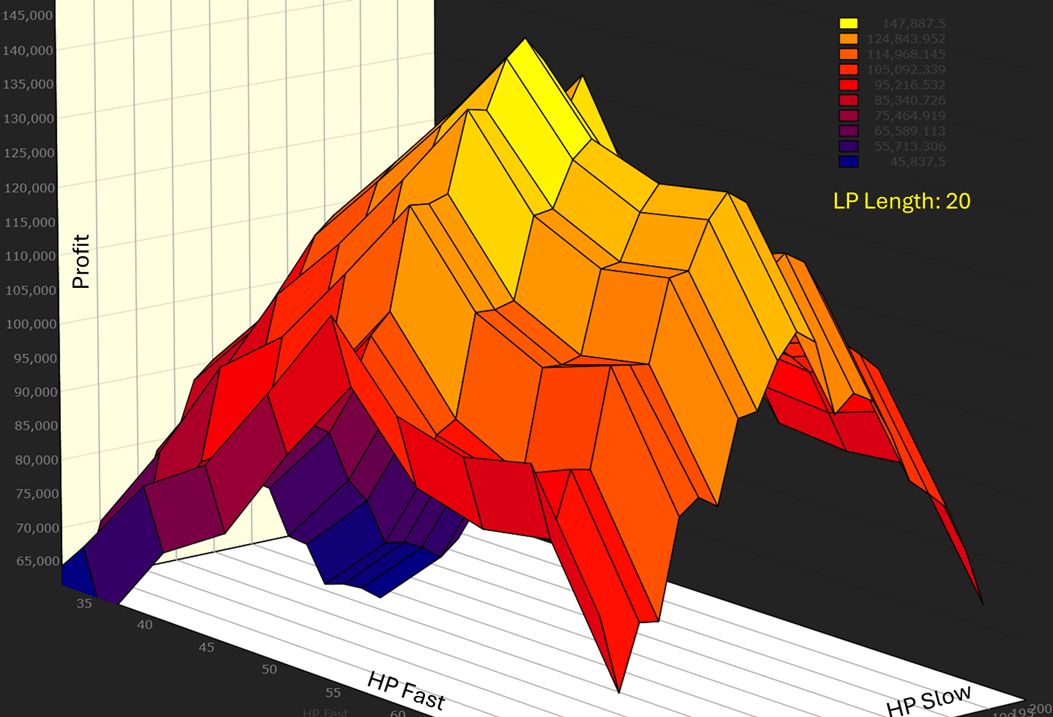
The code provided in the article didn’t use CyberneticOsc’s RMS version, but the result would likely be similar. Position sizing appears to have been one fixed contract for the entire backtest. The result would be far more profitable (and volatile) if contracts were sized proportionally with backtest buying power. Sizing aside, we ran our own quick optimization, changing parameter values in steps of 5. When judging if a system is stable, you want to see an optimization space like the one shown in Figure 2—a relatively smooth rolloff around an optimum, the peak, which represents the parameters used for the article.
using System;
using WealthLab.Backtest;
using WealthLab.Core;
using WealthLab.Indicators;
using WealthLab.TASC;

namespace WealthScript8
{
    public class CyberneticSystem : UserStrategyBase
    {
        Parameter _LPLength, _HPFast, _HPSlow;
        Momentum _mo1, _mo2;

        public CyberneticSystem()
        {
            _LPLength = AddParameter("LP Length", ParameterType.Int32, 20, 15, 30, 5);
            _HPFast = AddParameter("HP Fast", ParameterType.Int32, 55, 30, 75, 5);
            _HPSlow = AddParameter("HP Slow", ParameterType.Int32, 155, 100, 200, 5);
            StartIndex = _HPSlow.AsInt;
        }

        public override void Initialize(BarHistory bars)
        {
            //create and plot indicators
            SuperSmoother LP = new(bars.Close, _LPLength.AsInt);
            HighPass BP1 = new(LP, _HPFast.AsInt);
            HighPass BP2 = new(LP, _HPSlow.AsInt);

            _mo1 = new Momentum(BP1, 2);
            _mo2 = new Momentum(BP2, 2);
            PlotIndicatorLine(_mo1, WLColor.Green);
            PlotIndicatorLine(_mo2, WLColor.Red);
            DrawHorzLine(0, WLColor.White, 1, LineStyle.Dashed, _mo1.PaneTag);
        }

        public override void Execute(BarHistory bars, int idx)
        {
            //trading rules
            if (!HasOpenPosition(bars, PositionType.Long))
            {
                if (_mo1[idx] > 0 && _mo2[idx] > 0)
                    PlaceTrade(bars, TransactionType.Buy, OrderType.Market);
            }
            else
            {
                Position p = LastPosition;
                if (_mo1[idx] < 0 || _mo2[idx] < 0)
                    ClosePosition(p, OrderType.Market);
            }
        }
    }
}

FIGURE 2: WEALTH-LAB. This demonstrates a 3D optimization in Wealth-Lab output from the example trading strategy. This 3D optimization display is designed to help the user see whether a trading strategy is stable. In this case, a relatively smooth rolloff around an optimum at the peak such as this is a good sign.
—Robert Sucher
Wealth-Lab team
www.wealth-lab.com
BACK TO LIST

NinjaTrader: June 2025
In “Making A Better Oscillator” in this issue, John Ehlers presents a new oscillator he calls the cybernetic oscillator. The indicator discussed in the article is available for download at the following link for NinjaTrader 8:
Once the file is downloaded, you can import the indicator into NinjaTrader 8 from within the control center by selecting Tools → Import → NinjaScript Add-On and then selecting the downloaded file for NinjaTrader 8.
You can review the indicator source code in NinjaTrader 8 by selecting the menu New → NinjaScript Editor → Indicators folder from within the control center window and selecting the file.
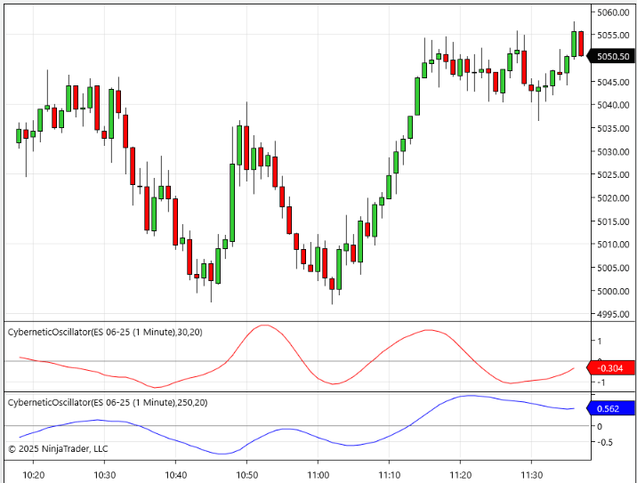
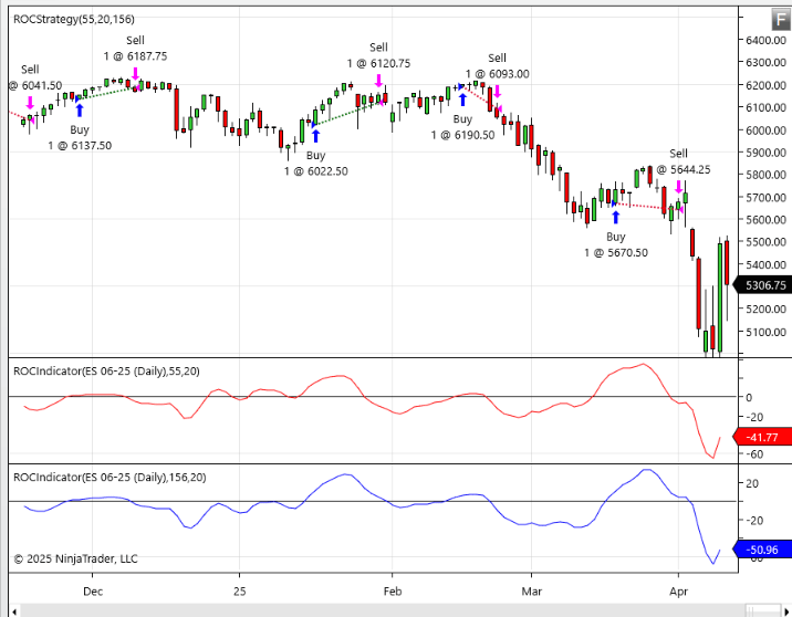
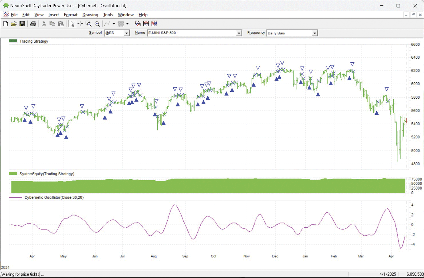
A sample chart demonstrating applying the cybernetic oscillator on a chart of ES is shown in Figure 3. Figure 4 demonstrates application of the author’s example trading strategy based on rate-of-change.

FIGURE 3: NINJATRADER. The cybernetic oscillator indicator is applied to a daily chart of ES.

FIGURE 4: NINJATRADER. The author’s example rate-of-change (ROC) strategy is demonstrated on a daily chart of ES.
NinjaScript uses compiled DLLs that run native, not interpreted, to provide you with the highest performance possible.
— Helom S.
NinjaTrader, LLC
www.ninjatrader.com
BACK TO LIST

RealTest: June 2025
Provided here is coding for use in the RealTest platform to create and plot the cybernetic oscillator indicator introduced in John Ehlers’ article in this issue, “Making A Better Oscillator.” The second listing codes the example strategy from the article.
Notes:
	John Ehlers "Cybernetic Oscillator", TASC, June 2025
	Implements and plots the indicators as in the article

Import:
	DataSource:	Norgate
	IncludeList:	&ES
	StartDate:	2023-01-01
	EndDate:	2025-04-01
	SaveAs:	es.rtd

Settings:
	DataFile:	es.rtd
	BarSize:	Daily

Parameters:
	HPLength:	30
	SSLength:	20
	RMSlen:	100

Data:
	// Common constants
	decay_factor:	-1.414 * 3.14159
	phase_angle:	1.414 * 180

	// Highpass Filter of Close
	hp_a1:	exp(decay_factor / HPLength)
	hp_b1:	2 * hp_a1 * Cosine(phase_angle / HPLength)
	hp_c2:	hp_b1
	hp_c3:	-hp_a1 * hp_a1
	hp_c1:	(1 + hp_c2 - hp_c3) / 4
	HPC:	if(BarNum >= 4, hp_c1 * (Close - 2 * Close[1] + Close[2]) + hp_c2 * HPC[1] + hp_c3 * HPC[2], 0)

	// SuperSmoother of HPC
	ss_a1:	exp(decay_factor / SSLength)
	ss_b1:	2 * ss_a1 * Cosine(phase_angle / SSLength)
	ss_c2:	ss_b1
	ss_c3:	-ss_a1 * ss_a1
	ss_c1:	(1 - ss_c2 - ss_c3)
	SSHPC:	if(BarNum >= 4, ss_c1 * (HPC + HPC[1]) / 2 + ss_c2 * SSHPC[1] + ss_c3 * SSHPC[2], HPC)

	// RMS of SSHPC
	RMS_SSHPC:	Sqr(SumSQ(SSHPC, RMSLen) / RMSLen)

	// Cybernetic Oscillator
	CyberneticOsc:	SSHPC / RMS_SSHPC

Charts:
	CyberneticOsc:	CyberneticOsc {|}
Notes:
	John Ehlers "Simple ROC Strategy", TASC, June 2025

Import:
	DataSource:	Norgate
	IncludeList:	&ES
	StartDate:	2009-01-01
	EndDate:	2025-01-01
	SaveAs:	es.rtd

Settings:
	DataFile:	es.rtd
	BarSize:	Daily
	StartDate:	2010-01-01
	EndDate:	Latest

Parameters:
	SSLength:	20
	FastHPLength:	55
	SlowHPLength:	156

Data:
	// Common constants
	decay_factor:	-1.414 * 3.14159
	phase_angle:	1.414 * 180

	// SuperSmoother of Close
	ss_a1:	exp(decay_factor / SSLength)
	ss_b1:	2 * ss_a1 * Cosine(phase_angle / SSLength)
	ss_c2:	ss_b1
	ss_c3:	-ss_a1 * ss_a1
	ss_c1:	(1 - ss_c2 - ss_c3)
	SSC:	if(BarNum >= 4, ss_c1 * (Close[1] + Close[2]) / 2 + ss_c2 * SSC[1] + ss_c3 * SSC[2], Close)

	// Fast Highpass Filter of SSC
	fhp_a1:	exp(decay_factor / FastHPLength)
	fhp_b1:	2 * fhp_a1 * Cosine(phase_angle / FastHPLength)
	fhp_c2:	fhp_b1
	fhp_c3:	-fhp_a1 * fhp_a1
	fhp_c1:	(1 + fhp_c2 - fhp_c3) / 4
	FHPSS:	if(BarNum >= 4, fhp_c1 * (SSC - 2 * SSC[1] + SSC[2]) + fhp_c2 * FHPSS[1] + fhp_c3 * FHPSS[2], 0)
	ROC1:	FHPSS - FHPSS[2]

	// Slow Highpass Filter of SSC
	shp_a1:	exp(decay_factor / SlowHPLength)
	shp_b1:	2 * shp_a1 * Cosine(phase_angle / SlowHPLength)
	shp_c2:	shp_b1
	shp_c3:	-shp_a1 * shp_a1
	shp_c1:	(1 + shp_c2 - shp_c3) / 4
	SHPSS:	if(BarNum >= 4, shp_c1 * (SSC - 2 * SSC[1] + SSC[2]) + shp_c2 * SHPSS[1] + shp_c3 * SHPSS[2], 0)
	ROC2:	SHPSS - SHPSS[2]

Strategy: Dual_ROC
	Side:	Long
	Quantity:	1
	EntrySetup:	ROC1 > 0 and ROC2 > 0
	ExitRule:	ROC1 < 0 or ROC2 < 0
—Marsten Parker
MHP Trading
mhp@mhptrading.com
BACK TO LIST

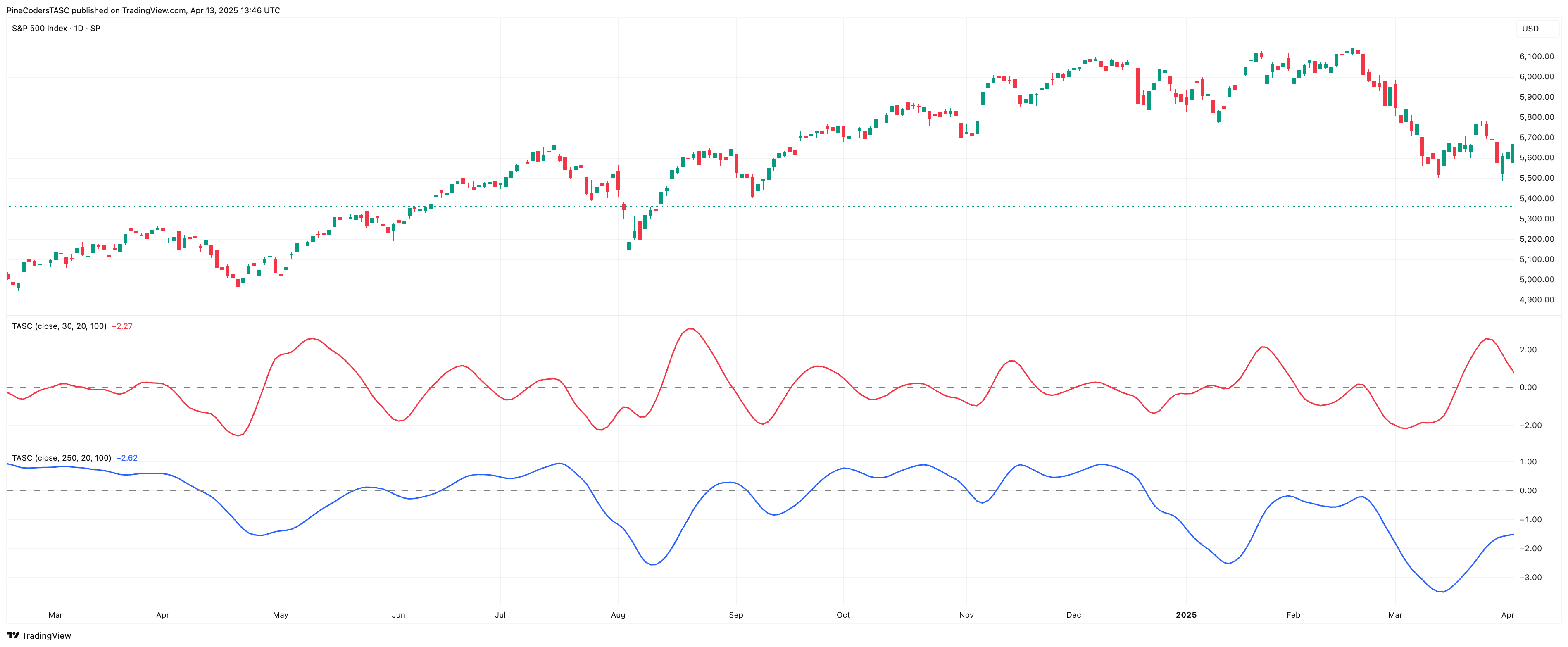
TradingView: June 2025
This TradingView Pine Script code provided here implements the cybernetic oscillator introduced by John Ehlers in his article in this issue, “Making A Better Oscillator.”
//  TASC Issue: June 2025
//     Article: The Cybernetic Oscillator For More Flexibility
//              Making A Better Oscillator
//  Article By: John F. Ehlers
//    Language: TradingView's Pine Script® v6
// Provided By: PineCoders, for tradingview.com


//@version=6
title ='TASC 2025.06 Making A Better Oscillator'
stitle = 'Making A Better Oscillator'
indicator(title, stitle, false)


//Inputs:


float src = input.source(close, 'Source Series:')
int HPLength = input.int(30, 'High Pass Length:')
int LPLength = input.int(20, 'Low Pass Length:')
int RMSLength = input.int(100, 'RMS Length:')


//Functions:


// @function High Pass Filter.
HP (float Source, int Period) =>
    var float hp = 0.0
    var float a0 = math.pi * 1.414 / Period
    var float a1 = math.exp(-a0)
    var float c2 = 2.0 * a1 * math.cos(a0)
    var float c3 = -a1 * a1
    var float c1 = (1.0 + c2 - c3) * 0.25
    if bar_index >= 4
        hp := c1 * (Source - 2.0 * Source[1] + Source[2]) +
              c2 * nz(hp[1]) +
              c3 * nz(hp[2])
    hp


// @function Super Smoother.
SS (float Source, int Period) =>
    var float ss = Source
    var float a0 = math.pi *  1.414 / Period
    var float a1 = math.exp(-a0)
    var float c2 = 2.0 * a1 * math.cos(a0)
    var float c3 = -a1 * a1
    var float c1 = 1.0 - c2 - c3
    if bar_index >= 4
        ss := c1 * ((Source + Source[1]) / 2.0) +
              c2 * nz(ss[1]) +
              c3 * nz(ss[2])
    ss


// @function Root Mean Square.
RMS (float Source, int Length) =>
    var float rms = 0
    float s2 = math.sum(Source * Source, Length)
    if s2 != 0
        rms := math.sqrt(s2 / Length)
    rms


// @function Cybernetic Oscillator.
CO (float Source, int HPLength=30, int LPLength=20,
 int RMSLength=100) =>
    var float co = 0
    float HP = HP(Source, HPLength)
    float LP = SS(HP, LPLength)
    float RMS = RMS(LP, RMSLength)
    if RMS != 0
        co := LP / RMS
    co


//Calculations:
float CO = CO(src, HPLength, LPLength, RMSLength)


//Plot + Zero Line:
plot(CO, 'Cybernetic Oscillator', color.blue)
hline(0)
The indicator is available for TradingView from the PineCodersTASC account: https://www.tradingview.com/u/PineCodersTASC/#published-scripts.
An example chart is shown in Figure 5.

FIGURE 5: TRADINGVIEW. Here you an example of John Ehlers’ cybernetic oscillator plotted on a daily chart of the S&P 500 index.
—PineCoders, for TradingView
www.TradingView.com
BACK TO LIST

Neuroshell Trader: June 2025
The John Ehlers’ cybernetic oscillator, highpass filter, and SuperSmoother can be easily implemented in NeuroShell Trader using NeuroShell Trader’s ability to call external dynamic linked libraries. Dynamic linked libraries can be written in C, C++ and Power Basic.
After moving the code given in the article to your preferred compiler and creating a DLL, you can insert the resulting indicator(s) as follows:
- Select “New indicator...” from the insert menu.
- Choose the External Program & Library Calls category.
- Select the appropriate External DLL Call indicator.
- Setup the parameters to match your DLL.
- Select the finished button.
To create a rotation trading system on a chart with a chart page for each of the two ETFs, select “New trading strategy” from the insert menu and enter the following in the appropriate locations of the trading strategy wizard:
BUY LONG CONDITIONS: [All of which must be true]
     A>B(Momentum(High Pass Filter(Super Smoother(Close,20),55),2),0)
     A>B(Momentum(High Pass Filter(Close,156),2),0)
SELL LONG CONDITIONS: [1 of which must be true]
     A<B(Momentum(High Pass Filter(Super Smoother(Close,20),55),2),0)
     A<B(Momentum(High Pass Filter(Close,156),2),0)
After entering the system conditions, you can also choose whether the parameters should be optimized. After backtesting the trading strategy, use the “Detailed analysis” button to view the backtest and trade-by-trade statistics for the system.
Figure 6 shows a chart plotting the cybernetic oscillator. It also shows the strategy.

FIGURE 6: NEUROSHELL TRADER. This NeuroShell Trader chart demonstrates the cybernetic oscillator and the simple dual ROC strategy, which is a simple strategy used only to demonstrate incorporating the oscillator into a trading strategy.
Users of NeuroShell Trader can go to the Stocks & Commodities section of the NeuroShell Trader free technical support website to download a copy of this or any previous Traders’ Tips.
—Ward Systems Group, Inc.
sales@wardsystems.com
www.neuroshell.com
BACK TO LIST

The Zorro Project: June 2025
Oscillator-type indicators swing around the zero line. They are often used for opening positions when the oscillator exceeds a positive or negative threshold. Continuing with his recent series of articles about no-lag or reduced-lag indicators, in this issue in his article titled “Making A Better Oscillator,” John Ehlers introduces an indicator he calls the cybernetic oscillator.
The cybernetic oscillator is built by applying a highpass and afterwards a lowpass filter to the price curve, then normalizing the result.
We are already familiar with Ehlers’ highpass filter from his previous articles, and so you can find it already in the Zorro indicator library under the name HighPass3. Meanwhile, the lowpass filter, which Ehlers calls the SuperSmoother, is also in the Zorro indicator library, as well as the sum of squares function for normalizing. Having these indicators in the Zorro library already makes the cybernetic oscillator easy to code in C:
var CyberOsc(vars Data,int HPLength,int LPLength)
{
  vars HP = series(HighPass3(Data,HPLength));
  vars LP = series(Smooth(HP,LPLength));
  var RMS = sqrt(SumSq(LP,100)/100);
  return LP[0]/fix0(RMS);
}
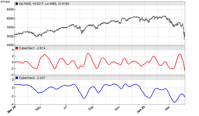
We can apply two cybernetic oscillators, one with a short and one with a long highpass cutoff, to an S&P 500 chart from 2024 using the following code in Zorro:
void run()
{
  BarPeriod = 1440;
  LookBack = 250;
  StartDate = 20240301;
  EndDate = 20250407;
  asset("SPX500");
  plot("CyberOsc1",CyberOsc(seriesC(),30,20),NEW|LINE,RED);
  plot("CyberOsc2",CyberOsc(seriesC(),250,20),NEW|LINE,BLUE);
}
The resulting chart, shown in Figure 7, replicates Ehlers’ chart in his article in this issue. The red line reproduces the swings of the price curve, the blue line the long-term trend.

FIGURE 7: ZORRO. Here is an example of the cybernetic oscillator plotted on a chart of the S&P 500. The red line reproduces the swings of the price curve, while the blue line is the long-term trend.
The oscillator could be used in trading, for example, by opening a swing position in the direction of the trend. In his article in this issue, Ehlers offers a simple trading strategy for the purpose of demonstrating incorporating the cybernetic oscillator. Here is code in C to do that in Zorro, converted from the EasyLanguage script that Ehlers provides in his article:
function run()
{
  BarPeriod = 1440;
  LookBack = 250;
  StartDate = 2009;
  EndDate = 2025;
  Fill = 2; // enter at next open
  assetList("AssetsIB"); // simulate IBKR
  asset("SPY");
  vars LP = series(Smooth(seriesC(),20));
  vars BP1 = series(HighPass3(LP,55));
  var ROC1 = BP1[0] - BP1[2];
  vars BP2 = series(HighPass3(LP,156));
  var ROC2 = BP2[0] - BP2[2];
  if(!NumOpenLong && ROC1 > 0 && ROC2 > 0)
    enterLong();
  if(NumOpenLong && (ROC1 < 0 || ROC2 < 0))
    exitLong();
}
Backtesting the same system with walk-forward optimization is left as an exercise to the reader.
The code can be downloaded from the 2025 script repository on https://financial-hacker.com. The Zorro platform can be downloaded from https://zorro-project.com.
—Petra Volkova
The Zorro Project by oP group Germany
https://zorro-project.com
BACK TO LIST
Python: June 2025
The Python code presented here is based on John Ehlers’ article in this issue, “Making A Better Oscillator,” which introduces his new cybernetic oscillator.
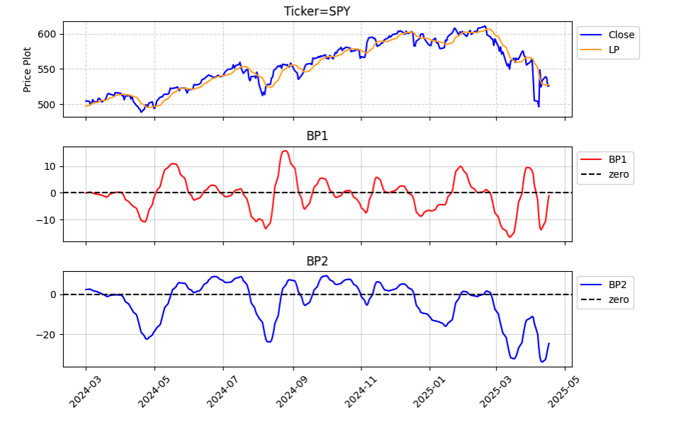
The routines given here perform tasks related to implementing the cybernetic oscillator using the Python language. This includes: importing the required python libraries; obtaining OHLCV data by using the Yahoo Finance Python package; using panda’s built-in plotting function to display a price chart; building blocks to build the cybernetic oscillator indicator; using MatPlotLib to plot close, CO1 and CO2 values; and finally, a callable routine to implement an example trading strategy based on rate-of-change, as described in Ehlers’ article.
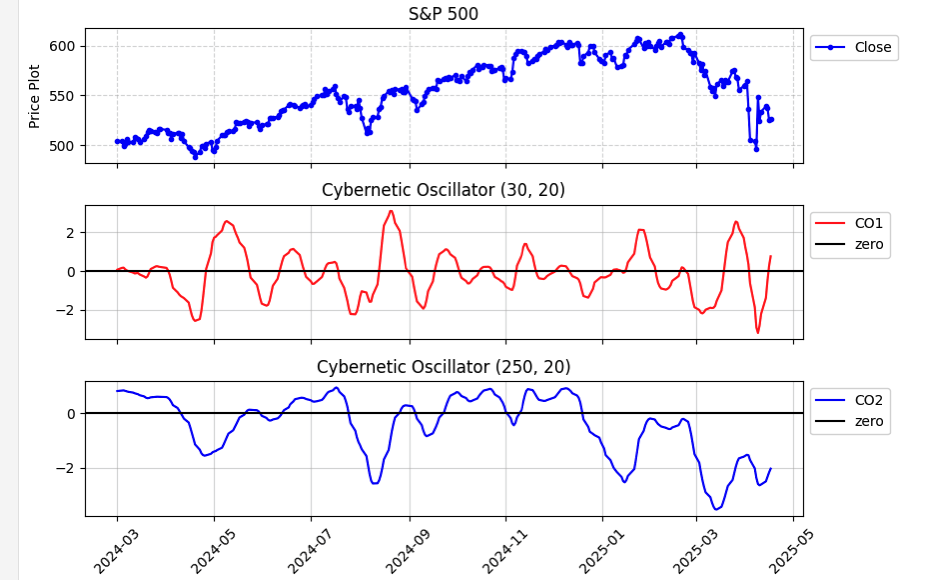
An example chart plotting both a long-term and short-term cybernetic oscillator is shown in Figure 8. A chart illustrating the creation of an example rate-of-change strategy is shown in Figure 9.

FIGURE 8: PYTHON. John Ehlers’ cybernetic oscillator is demonstrated here on a daily chart of the S&P 500. A short and longer-trend version are shown.

FIGURE 9: PYTHON. An example trading strategy incorporating the cybernetic oscillator is created for demonstration purposes. The strategy is a simple dual ROC strategy. The indicators are visualized using the MatplotLib routine. Here, LP, BP1, and BP2 can be observed along with price.
#
# import required python libraries
#
%matplotlib inline
import pandas as pd
import numpy as np
import matplotlib.pyplot as plt
import yfinance as yf
import math
import datetime as dt
print(yf.__version__)
#
# Use Yahoo Finance python package to obtain OHLCV data
#
symbol = '^GSPC'
symbol = 'SPY'
ohlcv = yf.download(symbol, start="1995-01-01", end="2025-04-18", group_by="Ticker", auto_adjust=True)
ohlcv = ohlcv[symbol]
#
# Use pandas built in plot function to see simple price chart
#
ax = ohlcv['Close'].plot(
figsize=(9,6),
grid=True,
title=f'{symbol}',
#marker='.'
)
#
# Building block / routines used to implement cybernetic oscillaor indicator
#
def calc_highpass(price, period):
a1 = np.exp(-1.414 * np.pi / period)
b1 = 2 * a1 * np.cos(math.radians(1.414 * 180 / period))
c2 = b1
c3 = -a1 * a1
c1 = (1 + c2 - c3)/4
out_values = []
for i in range(len(price)):
if i >= 4:
out_values.append(
c1*(price[i] - 2*price[i-1] + price[i-2]) + c2*out_values[i-1] + c3*out_values[i-2]
)
else:
out_values.append(price[i])
return out_values
def calc_super_smoother(price, period):
a1 = np.exp(-1.414 * np.pi / period)
b1 = 2 * a1 * np.cos(math.radians(1.414 * 180 / period))
c2 = b1
c3 = -a1 * a1
c1 = (1 - c2 - c3)
out_values = []
for i in range(len(price)):
if i >= 4:
out_values.append(c1*(price[i]+price[i-1])/2 + c2*out_values[i-1] + c3*out_values[i-2])
else:
out_values.append(price[i])
return out_values
def calc_rms(price):
length = len(price)
sum_sq = 0
for count in range(length):
sum_sq += price[count] * price[count]
return np.sqrt(sum_sq / length)
def calc_cybernetic_oscillator(close, params=(30, 20)):
hp_length = params[0]
lp_length = params[1]
df = pd.DataFrame(index=close.index, data=close)
df['HP'] = calc_highpass(close, hp_length)
df['LP'] = calc_super_smoother(df['HP'], lp_length)
df['RMS'] = df['LP'].rolling(100).apply(calc_rms)
df['CO'] = df['LP']/df['RMS']
return df['CO']
#
# Exampe python code to create two versions of the cybernetic oscillator
# as presented in June 2005 Trader Tip article
#
lp_length = 20
hp1_length = 30
hp2_length = 250
co1_params=(hp1_length, lp_length)
co2_params=(hp2_length, lp_length)
df = ohlcv.copy()
df['CO1'] = calc_cybernetic_oscillator(ohlcv['Close'], params=co1_params)
df['CO2'] = calc_cybernetic_oscillator(ohlcv['Close'], params=co2_params)
df
#
# MatPlotLib routine to plot Close, CO1 and CO2 values
#
def plot_indicators1(df):
# Create a figure with three subplots stacked vertically
fig, (ax1, ax2, ax3) = plt.subplots(3, 1, figsize=(9, 6), sharex=True)
# Plotting the first subplot (e.g., Price Data)
ax1.set_title(f"S&P 500")
ax1.plot(df.index, df['Close'], label='Close', color='blue', marker='.')
ax1.grid(True, linestyle='--', alpha=0.5)
ax1.set_ylabel('Price Plot')
ax1.legend(loc='upper left', bbox_to_anchor=(1, 1))
# Plotting the second subplot
ax2.set_title(f'Cybernetic Oscillator {co1_params}')
ax2.plot(df.index, df['CO1'], label='CO1', color='red')
ax2.axhline(y=0, color='black', linestyle='-', label='zero')
#ax2.set_ylabel('Linear Slope')
ax2.grid(True, linestyle='-', alpha=0.5)
ax2.legend(loc='upper left', bbox_to_anchor=(1, 1))
# Plotting the third subplot
ax3.set_title(f'Cybernetic Oscillator {co2_params}')
ax3.plot(df.index, df['CO2'], label='CO2', color='blue')
ax3.axhline(y=0, color='black', linestyle='-', label='zero')
ax3.grid(True, linestyle='-', alpha=0.5)
ax3.legend(loc='upper left', bbox_to_anchor=(1, 1))
# Rotate x-axis labels for better readability
plt.xticks(rotation=45)
# Improve overall layout
plt.tight_layout()
# Show the plot
plt.show()
plot_indicators1(df['2024-03':'2025'])
#
# Example python code to implement the simple dual ROC strategy showcased
# in trader tip article the python code is bundled in a *strategy* routine
# so it can easily be called, paramater as passed into the routine as a variable
#
def strategy(ohlcv, params):
df = ohlcv.copy()
df['LP'] = calc_super_smoother(df['Close'], params[0])
df['BP1'] = calc_highpass(df['LP'],params[1] )
df['ROC1'] = df['BP1'] - df['BP1'].shift(2)
df['BP2'] = calc_highpass(df['LP'],params[2])
df['ROC2'] = df['BP2'] - df['BP2'].shift(2)
df['Signal'] = np.where((df['ROC1'] > 0 ) & (df['ROC2'] >0 ), 1, np.nan)
df['Signal'] = np.where((df['ROC1'] < 0 ) & (df['ROC2'] <0 ), 0, df['Signal'])
df['Signal'] = df['Signal'].fillna(method='ffill')
return df
params=(20, 55, 156)
data = strategy(ohlcv, params)
data
#
# The Simple Dual ROC strategy indicators are visualized in the MatplotLib
# routine below. Here LP, BP1 and BP2 can be see observed along with price
#
def plot_indicators2(df):
# Create a figure with three subplots stacked vertically
fig, (ax1, ax2, ax3) = plt.subplots(3, 1, figsize=(9, 6), sharex=True)
# Plotting the first subplot (e.g., Price Data)
ax1.set_title(f"Ticker={symbol}")
ax1.plot(df.index, df['Close'], label='Close', color='blue',)
ax1.plot(df.index, df['LP'], label='LP', color='orange', )
ax1.grid(True, linestyle='--', alpha=0.5)
ax1.set_ylabel('Price Plot')
ax1.legend(loc='upper left', bbox_to_anchor=(1, 1))
# Plotting the second subplot
ax2.set_title(f'BP1')
ax2.plot(df.index, df['BP1'], label='BP1', color='red')
ax2.axhline(y=0, color='black', linestyle='--', label='zero')
#ax2.set_ylabel('Linear Slope')
ax2.grid(True, linestyle='-', alpha=0.5)
ax2.legend(loc='upper left', bbox_to_anchor=(1, 1))
# Plotting the third subplot
ax3.set_title(f'BP2')
ax3.plot(df.index, df['BP2'], label='BP2', color='blue')
ax3.axhline(y=0, color='black', linestyle='--', label='zero')
ax3.grid(True, linestyle='-', alpha=0.5)
ax3.legend(loc='upper left', bbox_to_anchor=(1, 1))
# Rotate x-axis labels for better readability
plt.xticks(rotation=45)
# Improve overall layout
plt.tight_layout()
# Show the plot
plt.show()
�plot_indicators2(data['2024-03':'2025'])
#
# A simple backtest framework/routines are provided which allow changing
# parameters and visualize performance results. Performance can be compared
# against Buy&Hold of same ticker by setting. All buy and sell occur on the
# day of the buy/sell signal using market close values
#
def backtest(data):
df = data.copy()
df['Return Ratio'] = np.where(df['Signal'].shift()==1, 1+df['Close'].pct_change(),1 )
df['Strategy'] = df['Return Ratio'].cumprod()
df['BH'] = (1+df['Close'].pct_change()).cumprod()
df['Peak'] = df['Strategy'].cummax()
df['% DD'] = 100*(df['Strategy']/df['Peak']-1)
df['Peak'] = df['BH'].cummax()
df['BH % DD'] = 100*(df['BH']/df['Peak']-1)
df.at[df.index[0], 'Strategy'] = 1
df.at[df.index[0], 'BH'] = 1
return df
def plot_backtest_results(df, strategy_name="Simple Dual ROC Strategy", compare_bh_ena=False):
fig, (ax1, ax2) = plt.subplots(2, 1, figsize=(9, 6), sharex=True)
ax1.set_title(f"{strategy_name}, Ticker={symbol},")
ax1.plot(df.index, df['Strategy'], label='Strategy Equity Curve', color='blue',)
if compare_bh_ena:
ax1.plot(df.index, df['BH'], label='Buy & Hold Equity Curve', color='orange',)
ax1.grid(True, linestyle='--', alpha=0.5)
ax1.set_ylabel('Cumulative Return')
ax1.legend(loc='upper left', bbox_to_anchor=(1, 1))
ax2.set_title(f"% Drawdown")
ax2.plot(df.index, df['% DD'], label='Strategy Drawdown', color='blue',)
if compare_bh_ena:
ax2.plot(df.index, df['BH % DD'], label='Buy & Hold Drawdown', color='orange',)
ax2.grid(True, linestyle='--', alpha=0.5)
ax2.set_ylabel('% drawdown')
ax2.legend(loc='upper left', bbox_to_anchor=(1, 1))
#
# Putting the building blocks toegther, parameters can be changed and results viewed visually
# Here using default values presenyed in article
#
params=(20, 55, 156)
data = strategy(ohlcv, params)
df = backtest(data['2009':'2024'])
plot_backtest_results(df, strategy_name="Simple Dual ROC Strategy", compare_bh_ena=False)
#
# Here change parameter and see results compared to buy & hold of same ticker
#
params=(50, 55, 156)
data = strategy(ohlcv, params)
df = backtest(data['2009':'2024'])
plot_backtest_results(df, compare_bh_ena=True)
—Rajeev Jain
jainraje@yahoo.com
BACK TO LIST
Microsoft Excel: June 2025
In his article in this issue, “Making A Better Oscillator,” John Ehlers combines a couple of the bits taken from his recent articles to build an oscillator where we can tune the upper and lower frequency limits of our band of interest. This allows tuning for swing or trend response at our option. He calls the new oscillator the cybernetic oscillator.
See Figure 10 for an example of the cybernetic oscillator plotted on a daily chart of the emini S&P 500 futures contract (ES), similar to Figure 4 in Ehlers’ article in this issue.

FIGURE 10: EXCEL. Two versions of the cybernetic oscillator are plotted here on a daily chart of the emini S&P 500 futures contract (ES), one using parameters for longer trends and one using parameters for shorter timeframes.
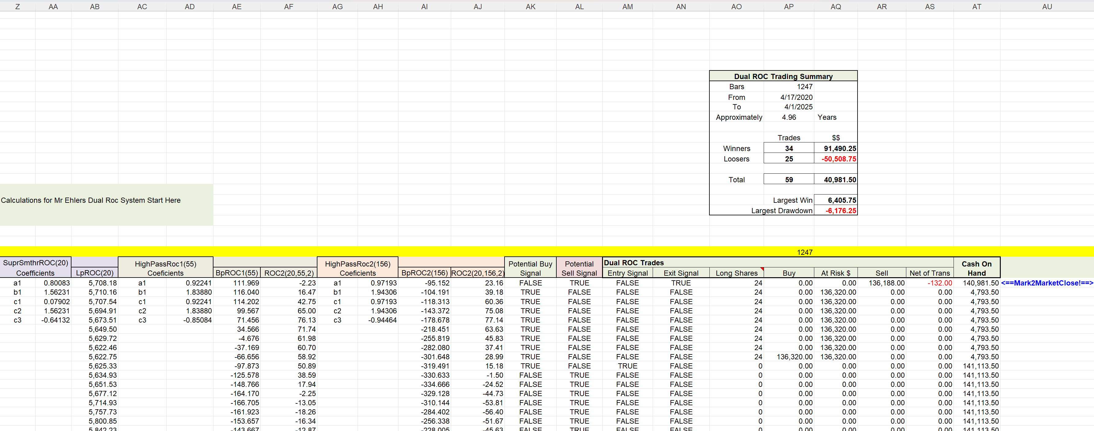
In the article, Ehlers also provides a simple trading strategy to demonstrate using the oscillator. The trading system is built by comparing the rate of change (ROC) of two cybernetic oscillators with slightly different band specifications. In Figure 11 I show an example of recent trades based on this strategy. The lower charts in Figure 2 track the individual ROC values. When both ROC values go positive, it produces a buy signal and when either ROC value goes negative, it produces a sell signal. The green and red dots mark when these conditions are true. The green and red shading highlight the price bars involved in trades. Scrolling the CalculationsAndChart tab right to column Z (Figure 12) reveals the calculations to trade using this dual ROC strategy. As noted in the summary block, calculations in this spreadsheet cover almost five years, enough to demonstrate the simple strategy.

FIGURE 11: EXCEL. Here is the example trading strategy, the dual ROC strategy. The strategy enters when both ROC values are positive and exits when either ROC goes negative. Winners and losers are highlighted on the price chart.

FIGURE 12: EXCEL. To view the dual ROC trading strategy calculations, scroll right to column Z.
To download this spreadsheet: The spreadsheet file for this Traders’ Tip can be downloaded here. To successfully download it, follow these steps:
- Right-click on the Excel file link, then
- Select “save as” (or “save target as”) to place a copy of the spreadsheet file on your hard drive.
P.S. For anyone using 32-bit Excel, the “REPAIRS” tab in this spreadsheet is now capable of tailoring repairs according to the “bit-ness” of the running Excel.
—Ron McAllister
Excel and VBA programmer
rpmac_xltt@sprynet.com
BACK TO LIST
Originally published in the June 2025 issue of
Technical Analysis of STOCKS & COMMODITIES magazine.
All rights reserved. © Copyright 2025, Technical Analysis, Inc.


