TRADERS’ TIPS
May 2025

For this month’s Traders’ Tips, the focus is Perry J. Kaufman’s article in this issue, “Trading The Channel.” Here, we present the May 2025 Traders’ Tips code with possible implementations in various software.
You can right-click on any chart to open it in a new tab or window and view it at it’s originally supplied size, often much larger than the version printed in the magazine.
The Traders’ Tips section is provided to help the reader implement a selected technique from an article in this issue or another recent issue. The entries here are contributed by software developers or programmers for software that is capable of customization.

TradeStation: May 2025
In “Trading The Channel” in this issue, Perry Kaufman explores trading bands (channels), covering three approaches: trend trading, breakout trading, and shorter-term trades within the channel. The EasyLanguage strategy code we are providing utilizes Kaufman’s “PJK channels” code provided in his article accompanied by two functions. The rule input determines which approach to use. It can be set to 1, 2, or 3. See the code comments for details on how its value affects the logic.
Strategy: PJK Channels
[LegacyColorValue = true];
{
	TASC MAY 2024
	PJK Channels
	Copyright 2024–2025, P.J. Kaufman.
	All rights reserved.
}
{ period = calculation period
Rule = 0,1 use slope for trend only
	 = 2, create bands, exit on break of band
 		band based on high-low deviation
	 = 3, enter on lower band, exit at top band
		need % zone
DataOption  = 1, use close
			= 2, use (high + low + close)/3
 			= 3, use (high + low)/2
}

inputs:
	Rule( 1 ),
	Period( 40 ),
	Zone( 0.20 ),
	DataOption( 1 ),
	UseFutures( false ),
	LongOnly( false ),
	PrintDetail( false ),
	DetailFile( "" );

variables:
	signal( 0 ),
	slope( 0 ),
	intercept( 0 ),
	size( 0 ),
	highdev( 0 ),
	lowdev( 0 ),
	linevalue( 0 ),
	deviation( 0 ),
	upperband( 0 ),
	lowerband( 0 ),
	price( 0 ),
	ix( 0 ),
	pricetarget( 0 ),
	stockinvestment( 100000 ),
	futuresinvestment( 25000 ),
	equity( 0 ),
	longprofit( 0 ),
	shortprofit( 0 ),
	adate( " " ),
	optimizing( GetAppInfo( aiOptimizing ) = 1 );

if DataOption = 1 then
    Price = Close
else if DataOption = 2 then
    Price = (High + Low + Close) / 3
else if DataOption = 3 then
    Price = (High + Low) / 2;

// Linear regression slope
slope = TSMLRslope(Price, Period);
Print( "Slope: ", Slope );

if slope > 0 then
    signal = 1
else if slope < 0 then
    signal = -1;

// for new positions
if UseFutures then
    size = futuresinvestment
     / (AvgTrueRange( 20 ) * BigPointValue)
else
    size = stockinvestment / Close;
 print( "Slope: ", Slope );
// rule 0/1 trend only using slope
if Rule <= 1 and signal <> signal[1] then
begin
    if MarketPosition <= 0 and signal = 1 then
    begin
        Buy to Cover all contracts this bar on Close;
        if UseFutures then
            Buy size contracts This Bar on Close
        else
            Buy size shares next bar on Open;
    end
    else if MarketPosition >= 0 and signal = -1 then
    begin
        Sell all contracts this bar on Close;
        if LongOnly = false then
            Sell Short size contracts This Bar on Close;
    end;
end;

// if rule > 1 create bands over period
intercept = TSMLRintercept(price, Period);
// find the highest and lowest deviation from the
// trend line
highdev = 0;
lowdev = 0;
for ix = 1 to Period
begin
    linevalue = intercept + slope * ix;
    deviation = Close[ix] - linevalue;
    highdev = MaxList(highdev, deviation);
    lowdev = MinList(lowdev, deviation);
end;
// value of bands today is last value in the loop above
upperband = linevalue + highdev;
lowerband = linevalue + lowdev;

// Rule 2, Buyon upwards band penetration of downward slope
if Rule = 2 then
begin
    // exit current position
    if MarketPosition > 0 and close < lowerband then
    begin
        if UseFutures then
            Sell ("XupBfut") all contracts
             this bar on Close
        else
            Sell ("XupBeq") all contracts
             next bar on Open;
    end
    else if MarketPosition < 0 and Close > upperband then
    begin
        if UseFutures then
            Buy to Cover ("XdnBfut") all contracts
             this bar on Close
        else
            Buy to Cover ("XdnBeq") all contracts
             next bar on Open;
    end;
    // set new position rule 2
    if MarketPosition <= 0 and Close > upperband then
    begin
        if UseFutures then
            Buy("BuyUBfut") size contracts
             this bar on Close
        else
            Buy("BuyUBstk") size shares
             next bar on Open;
    end;
    if MarketPosition >= 0 and close < lowerband then
    begin
        if UseFutures then
        begin
            Sell all contracts this bar on Close;
            if LongOnly = false then
                Sell short ("SellLBfut") size contracts
                 this bar on Close;
        end
        else
        begin
            Sell all shares next bar on Open;
            if LongOnly = false then
                Sell Short ("SellLBstk") size shares
                 next bar on Open;
        end;
    end;
end; {Rule 2}

// Rule 3: Trade within the bands
if Rule = 3 then
begin
    // exits first (should be intraday exit)
    if MarketPosition > 0 then
    begin
        pricetarget = upperband - Zone
         * (upperband - lowerband);
        if close >= pricetarget or slope < 0 then
            Sell ("L3exit") all contracts
             this bar on Close;
    end
    else if MarketPosition < 0 then
    begin
        pricetarget = lowerband + Zone
         * (upperband - lowerband);
        if close <= pricetarget or slope > 0 then
            Buy to Cover ("S3exit") all contracts
             this bar on Close;
    end;
    // new positions - trade in direction of slope
    if MarketPosition <= 0 and slope > 0 then
    begin
        Buy to Cover all contracts this bar on Close;
        pricetarget = lowerband + Zone
         * (upperband - lowerband);
        if Close <= pricetarget then
            Buy("L3entry") size contracts
             this bar on Close;
    end
    else if MarketPosition >= 0 and slope < 0 then
    begin
        Sell all contracts this bar on close;
        if longonly = false then
        begin
            pricetarget = upperband - Zone
             * (upperband - lowerband);
            if close >= pricetarget then
            begin
                Sell Short ("S3entry") size contracts
                 this bar on Close;
            end;
        end;
    end;
end; {end rule 3}

equity = NetProfit + OpenPositionProfit;

if MarketPosition > 0 then
    longprofit = longprofit + equity - equity[1]
else if MarketPosition < 0 then
    shortprofit = shortprofit + equity - equity[1];

adate = ELdatetostring( date );

if PrintDetail and optimizing = false then
begin
    if Currentbar = 1 then
    	print( file( "C:\TradeStation\PJK_Channel_Detail.csv" ),
     "Date,Open,High,Low,Close,Slope,Inter",
     "Lastvalue,HighDev,LowDev,UpBand,LowBand",
     "Signal,Shares,TodayPL,LongPL,ShortPL,TotalPL");

    print( file( "C:\TradeStation\PJK_Channel_Detail.csv" ),
     adate, ",", open:6:4, ",", high:6:4, ",", low:6:4, ",",
     close:6:4, ",", slope:6:4, ",", intercept:6:4, ",",
     linevalue:6:4, ",", highdev:6:4, ",", lowdev:6:4, ",",
     upperband:6:4, ",", lowerband:6:4, ",", signal:5:0, ",",
     currentcontracts:5:0, ",", equity-equity[1]:8:2, ",",
     longprofit:8:2, ",", shortprofit:8:2, ",", equity:8:2);
end;


Function: TSMLRIntercept
{
	TASC MAY 2025
	TSMLRintercept : Linear regression intercept
 	Copyright 1994-1999, 2021–2025 P.J. Kaufman.
 	All rights reserved.
 	Method of least squares to calculate slope
 }
{
	price = input series
 	period = length of calculation
}

 inputs:
 	price( numericseries ),
 	period( numericsimple );

 variables:
	sumx( 0 ),
	sumx2( 0 ),
	sumy( 0 ),
	sumxy( 0 ),
	n( 0 ),
	k( 0 ),
	top( 0 ),
	bot( 0 ),
 	slope( 0 ),
 	yint( 0 );

{ time = x, the independent variable, e.g., 1, 2, 3, ...
 price = y, the dependent variable }
{ standard sum of integer series }
sumx = period * (period + 1) / 2;
sumx2 = period * (period + 1) * (2 * period + 1) / 6;
sumy = Summation(price, period);
sumxy = 0;
n = period;

for k = 0 to period-1
begin
	sumxy = sumxy + n*price[k];
	n = n - 1;
end;

top = period*sumxy - sumx*sumy;
bot = period*sumx2 - sumx*sumx;
if bot <> 0 then
	slope = top / bot
else
	slope = 0;

TSMLRintercept = (sumy - slope*sumx) / period;


Function: TSMLRSlope
[LegacyColorValue = true];
{
	TASC MAY 2025
TSMLRslope : Linear regression slope
 Copyright 1994-2025, P.J. Kaufman. All rights reserved.
 Method of least squares to calculate slope }
{ price = input series
 period = length of calculation }
 inputs:
 	price(numericseries),
 	period(numericsimple);

 variables:
 	sumx(0),
 	sumx2(0),
 	sumy(0),
 	sumxy(0),
 	n(0),
 	k(0),
 	top(0),
	bot(0),
	slope(0),
	yint(0);
{ time = x, the independent variable, e.g., 1, 2, 3, ...
 price = y, the dependent variable }
{ standard sum of integer series }
 sumx = period * (period + 1) / 2;
 sumx2 = period * (period + 1) * (2 * period + 1) / 6;
 sumy = Summation(price, period);
 sumxy = 0;
 n = period;
 for k = 0 to period-1 begin
 sumxy = sumxy + n*price[k];
 n = n - 1;
 end;
 top = period*sumxy - sumx*sumy;
 bot = period*sumx2 - sumx*sumx;
 if bot <> 0 then
 slope = top / bot
 else
 slope = 0;
{ yint = (sumy - slope*sumx) / period; }
 TSMLRslope = slope;
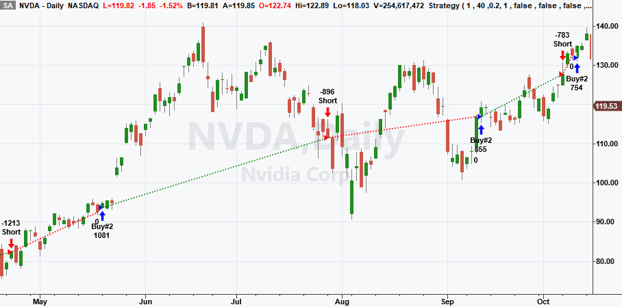
A sample chart is shown in Figure 1.

FIGURE 1: TRADESTATION. This demonstrates a daily chart of NVDA showing a portion of 2024 with the strategy applied.
This article is for informational purposes. No type of trading or investment recommendation, advice, or strategy is being made, given, or in any manner provided by TradeStation Securities or its affiliates.
—John Robinson
TradeStation Securities, Inc.
www.TradeStation.com
BACK TO LIST

Wealth-Lab.com: May 2025
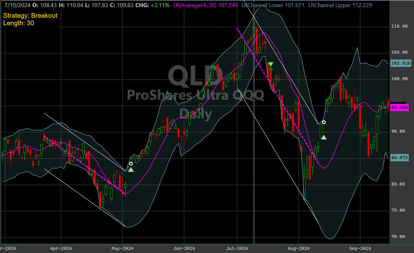
We’re providing code below based on Perry Kaufman’s article in this issue, “Trading The Channel.” Using the first strategy parameter, WealthLab’s code switches between two of the strategies from Kaufman’s article—channel breakout and in-channel trading. For simplicity, we used all market orders, while the author’s code had logic that switched between market orders and at-the-close orders. In Figure 2, you’ll see the straight-line linear regression (LR) and channel lines plotted (another strategy parameter option) when a trade is triggered.

FIGURE 2: WEALTH-LAB. Here you see a straight-line linear regression (LR) and channel lines plotted on a daily chart of ProShares Ultra QQQ ETF (QLD). The endpoints of the linear regression line and channel lines form the LR series (in fuchsia) and bands.
using System;
using WealthLab.Backtest;
using WealthLab.Core;
using WealthLab.Data;
using WealthLab.Indicators;
using System.Collections.Generic;

namespace WealthScript3
{
	public class TASC202505 : UserStrategyBase
	{
		Parameter _strategy, _length, _chPct, _channelPlot;
		TimeSeries _source, _upperChnl, _lowerChnl;
		LR _linreg;
		LRSlope _lrSlope;

		public TASC202505()
		{
			_strategy = AddParameter("Strategy (hint)", ParameterType.Int32, 1, 0, 1);
			_strategy.Hint = "0 = In-Channel trading; 1 = Breakout";
			_length = AddParameter("LR Length", ParameterType.Int32, 20, 20, 150, 10);
			_chPct = AddParameter("Channel Width %", ParameterType.Double, 5, 0, 50, 5);
			_channelPlot = AddParameter("Plot Channels", ParameterType.Int32, 0, 0, 1);
		}

		public override void Initialize(BarHistory bars)
		{
			//Create and plot the LR line and channel
			NewWFOInterval(bars);
			string st = _strategy.AsInt == 1 ? "Breakout" : $"In-Channel ({_chPct.AsDouble:N1}%)";
			DrawHeaderText($"Strategy: {st}\nLength: {_length.AsInt}", WLColor.Gold, 14);
			PlotIndicatorLine(_linreg, WLColor.Fuchsia, 1);
			PlotTimeSeriesBands(_upperChnl, _lowerChnl, "LRChannel", "Price", WLColor.CadetBlue, 1, 15);
		}

		public override void NewWFOInterval(BarHistory bars)
		{
			int len = _length.AsInt;
			StartIndex = len;
			_source = _strategy.AsInt == 0 ? bars.AveragePriceHLC : bars.AveragePriceHL;
			_linreg = LR.Series(_source, len);
			_lrSlope = LRSlope.Series(_source, len);
			_upperChnl = new TimeSeries(bars.DateTimes);
			_lowerChnl = new TimeSeries(bars.DateTimes);

			//calculate channel band
			for (int bar = len; bar < bars.Count; bar++)
			{
				var lr = LinReg(bars.Close, bar, len);
				LRChannel(bars, bar, len, lr, out double U, out double L);
				_upperChnl[bar] = _linreg[bar] + U;
				_lowerChnl[bar] = _linreg[bar] + L;
			}
		}

		LinearRegression LinReg(TimeSeries ts, int bar, int length)
		{
			int bar0 = bar - length + 1;
			if (bar0 < 0 || length < 2)
				return null;

			List<double> data = new List<double>();
			for (int n = bar0; n <= bar; n++)
				data.Add(ts[n]);
			return new LinearRegression(data);
		}

		void LRChannel(BarHistory bars, int bar, int length, LinearRegression lr, out double U, out double L)
		{
			U = 0; L = 0;
			for (int i = 0; i < length - 1; i++)
			{
				double LRvalue = lr.PredictValue(length - i - 1);
				double d = bars.High[bar - i] - LRvalue;
				if (d > U) U = d;
				d = bars.Low[bar - i] - LRvalue;
				if (d < L) L = d;
			}
		}

		void PlotChannelLines(BarHistory bars, int bar)
		{
			int len = _length.AsInt;
			var lr = LinReg(_source, bar, len);
			int x = bar - _length.AsInt + 1;
			double U = _upperChnl[bar] - _linreg[bar];
			double L = _lowerChnl[bar] - _linreg[bar];
			DrawLine(x, lr.PredictValue(0), bar, lr.PredictValue(len - 1), WLColor.Fuchsia, 2, LineStyle.Dashed);
			DrawLine(x, lr.PredictValue(0) + U, bar, lr.PredictValue(len - 1) + U, WLColor.White, 1, LineStyle.Dashed);
			DrawLine(x, lr.PredictValue(0) + L, bar, lr.PredictValue(len - 1) + L, WLColor.White, 1, LineStyle.Dashed);
		}

		//strategy rules
		public override void Execute(BarHistory bars, int idx)
		{
			if (_strategy.AsInt == 1) // breakout strategy; long only
			{
				if (!HasOpenPosition(bars, PositionType.Long))
				{
					if (_lrSlope[idx] < 0 && bars.Close.CrossesOver(_upperChnl >> 1, idx))
						EnterAtMarket(bars, idx, TransactionType.Buy);
				}
				else
				{
					Position p = LastPosition;
					if (bars.Close.CrossesUnder(_lowerChnl >> 1, idx))
						ClosePosition(p, OrderType.Market);
				}
			}
			else // in channel strategy; long/short
			{
				double w = (_upperChnl[idx] - _lowerChnl[idx]) * _chPct.AsDouble / 100d;
				Position p = LastPosition;

				if (p == null || !p.IsOpen)
				{
					if (_lrSlope[idx] > 0) // long if trend (slope) is up
					{
						 if (bars.Close[idx] < _lowerChnl[idx] + w)
							EnterAtMarket(bars, idx, TransactionType.Buy);
					}
					else if (bars.Close[idx] > _upperChnl[idx] - w)
						EnterAtMarket(bars, idx, TransactionType.Short);
				}
				else  // exit, reverse only if trend direction changed
				{
					if (p.PositionType == PositionType.Long)
					{
						if (bars.Close[idx] > _upperChnl[idx] - w)
						{
							ClosePosition(p, OrderType.Market);
							if (_lrSlope[idx] < 0)
								EnterAtMarket(bars, idx, TransactionType.Short);
						}
					}
					else if (bars.Close[idx] < _lowerChnl[idx] + w)
					{
						ClosePosition(p, OrderType.Market);
						if (_lrSlope[idx] > 0)
							EnterAtMarket(bars, idx, TransactionType.Buy);
					}
				}
			}

			Transaction EnterAtMarket(BarHistory bars, int bar, TransactionType tt)
			{
				if (_channelPlot.AsInt == 1)
					PlotChannelLines(bars, bar - _strategy.AsInt);
				return PlaceTrade(bars, tt, OrderType.Market);
			}
		}
	}
}
—Robert Sucher
Wealth-Lab team
www.wealth-lab.com
BACK TO LIST

NinjaTrader: May 2025
In “Trading The Channel” in this issue, Perry Kaufman discusses several approaches to trading with a channel (trading bands). The technique discussed in the article is available for download at the following link for NinjaTrader 8:
Once the file is downloaded, you can import the file into NinjaTrader 8 from within the control center by selecting Tools → Import → NinjaScript Add-On and then selecting the downloaded file for NinjaTrader 8.
You can review the source code in NinjaTrader 8 by selecting the menu New → NinjaScript Editor → Indicators folder from within the control center window and selecting the file.
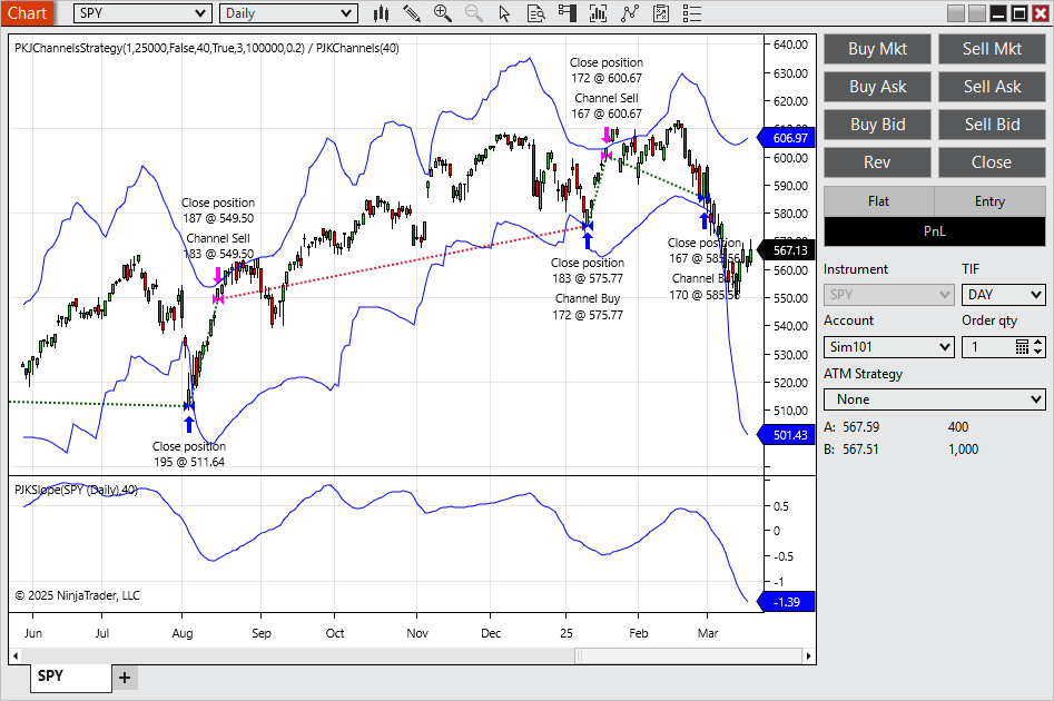
A sample chart is shown in Figure 3.

FIGURE 3: NINJATRADER. The author’s channel methods are demonstrated here on a daily chart of SPY.
NinjaScript uses compiled DLLs that run native, not interpreted, to provide you with the highest performance possible.
—Jesse N.
NinjaTrader, LLC
www.ninjatrader.com
BACK TO LIST

RealTest: May 2025
Provided here is coding for use in the RealTest platform to implement concepts described in Perry Kaufman’s article in this issue, “Trading The Channel.”
Notes:
	Perry Kaufman "Trading The Channel", TASC, May 2025

Import:
	DataSource:	Norgate
	IncludeList:	SPY, AAPL, NVDA {"stocks"}
	IncludeList:	&ZN_CCB, &CL_CCB {"futures"}
	StartDate:	1/1/10
	EndDate:	Latest
	SaveAs:	tasc_may_25.rtd

Settings:
	DataFile:	tasc_may_25.rtd
	StartDate:	Earliest
	EndDate:	Latest
	BarSize:	Daily
	AccountSize:	100000
	SkipTestIf:	rule <> 3 and zone <> 0.4 // skip redundant tests for rules that don't use zone

Parameters:
	rule:	from 1 to 3 def 3
	dataOption:	from 1 to 3 def 1 // 1 = use close, 2 = (high+low+close)/3, 3 = (high+low)/2
	period:	from 20 to 150 step 10 def 80
	zone:	from 0.05 to 0.5 step 0.05 def 0.4 // only relevant for rule 3

Data:
	// basic values
	stock:	InList("stocks")
	futures:	InList("futures")
	price:	Select(dataOption = 1, close, dataOption = 2, (high + low + close) / 3, dataOption = 3, (high + low) / 2)

	// linear regression
	lrSlope:	Slope(price, period)
	lrIntercept:	YInt(price, period)

	// high/low deviation calculation as described in the article text (different from code)
	// this subtracts each close from the corresponding LR point and calculates min and max deviations
//	highdev:	Highest(close - This(lrIntercept + funbar * lrSlope), period)
//	lowdev:	Lowest(close - This(lrIntercept + funbar * lrSlope), period)

	// high/low deviation calculation as implemented in article code (the "for ix = 1 to period" loop)
	// this subtracts oldest LR point from newest close (ignoring today), second-oldest LR from second-newest close, etc.
	// this surprising logic seems to produce better results than the above
	highdev:	Highest(close[1] - This(lrIntercept + (period - funbar) * lrSlope), period)
	lowdev:	Lowest(close[1] - This(lrIntercept + (period - funbar) * lrSlope), period)

	// slope signal (rules 1 and 3)
	signal:	sign(lrSlope)

	// deviation bands (rules 2 and 3)
	lrLine:	lrIntercept + lrSlope * period
	upperBand:	lrLine + highDev
	lowerBand:	lrLine + lowDev

	// band zones (rule 3)
	zoneWidth:	zone * (upperBand - lowerBand)
	priceTargetShort:	lowerBand + zoneWidth
	priceTargetLong:	upperBand - zoneWidth

// indicator plotting

Charts:
	// plot in price pane
	lrLine:	lrLine
	upperBand:	upperBand
	lowerBand:	lowerBand
	longTarget:	priceTargetLong
	shortTarget:	priceTargetShort

	// plot in lower pane
	lrSlope:	lrSlope {|}

// common strategy elements

Template: stocks
	Side:	Long
	Quantity:	100000
	QtyType:	Value
	EntryTime:	NextOpen
	ExitTime:	NextOpen

Template: futures
	Side:	Both
	Quantity:	signal * 25000 / (ATR(20) * PointValue)
	QtyType:	Shares // i.e. contracts
	EntryTime:	ThisClose
	ExitTime:	ThisClose

// strategy definitions

Strategy: pjk_rule1_stocks
	Using:	stocks
	EntrySetup:	rule = 1 and stock and lrSlope > 0
	ExitRule:	lrSlope < 0

Strategy: pjk_rule1_futures
	Using:	futures
	EntrySetup:	rule = 1 and futures and signal <> signal[1]
	ExitRule:	signal <> signal[1]

Strategy: pjk_rule2_stocks
	Using:	stocks
	EntrySetup:	rule = 2 and stock and close > upperBand
	ExitRule:	close < lowerBand

Strategy: pjk_rule2_futures
	Using:	futures
	EntrySetup:	rule = 2 and futures and (close > upperBand or close < lowerBand)
	ExitRule:	(side > 0 and close < lowerBand) or (side < 0 and close > upperBand)

// the author's code does not differentiate stocks vs. futures in rule3 but I did so here as per the other rules

Strategy: pjk_rule3_stocks
	Using:	stocks
	EntrySetup:	rule = 3 and stock and signal > 0 and close <= priceTargetShort // enter on pullback
	ExitRule:	signal < 0 or close >= priceTargetLong

Strategy: pjk_rule3_futures
	Using:	futures
	EntrySetup:	rule = 3 and futures and ((signal > 0 and close <= priceTargetShort) or ((signal < 0 and close >= priceTargetLong)))
	ExitRule:	signal <> side or (side > 0 and close >= priceTargetLong) or (side < 0 and close <= priceTargetLong)
—Marsten Parker
MHP Trading
mhp@mhptrading.com
BACK TO LIST

TradingView: May 2025
The Pine Script code for TradingView presented here enables traders to choose between the three approaches to trading channels discussed in Perry Kaufman’s article in this issue, “Trading The Channel.” The three approaches are: following the trend, trading breakouts, or trading within the channel. The author also uses a linear regression line.
//  TASC Issue: May 2025
// 	Article: A Test Of Three Approaches
//          	Trading The Channel
//  Article By: Perry J. Kaufman
//	Language: TradingView's Pine Script® v6
// Provided By: PineCoders, for tradingview.com

//@version=6
title ='TASC 2025.05 Trading The Channel'
stitle = 'Trading The Channel'
qtyt = strategy.fixed
strategy(title, stitle, false, default_qty_type=qtyt)

//@enum Trade Rules.
enum RULE
	T1 = 'Trade the trend.'
	T2 = 'Trade a channel breakout.'
	T3 = 'Trade within the channel.'

string TT1  = 'Recommended use of `close`, `hlc3` or `hl2`.'
string TT2  = 'Percent of Bands to use as trading zones.'
string TT3  = 'When "Trade within the channel."\n
 -> Only long when trend is up\n -> Only short when trend is down'

RULE rule   = input.enum(RULE.T1, 'Select Trade rule:')
int period  = input.int(40, 'Period:')
float price = input.source(close, 'Source:', tooltip=TT1)
float zone  = input.float(0.2, 'Zone %:', tooltip=TT2)
bool longonly = input.bool(false, 'Long Only?')
bool filter = input.bool(false, 'Extra filter "Trade within the channel."', tooltip=TT3)

// LRISS : Linear regression intercept, slope and signal
// @function Method of least squares to calculate
// linear regression intercept and slope.
// @param price Data Series Source.
// @param period Data window.
LRISS(float src, simple int length) =>
	var float sx  = length * (length + 1) / 2
	var float sxx = length * (length + 1) * (2 * length + 1) / 6
	var float sxy = 0.0
	float 	sy  = math.sum(src, length)
	float 	syy = math.sum(src * src, length)
	float  linreg = ta.linreg(price, period, 0)
	float  oldSrc = src[length]

	sxy += switch
    	bar_index <= length - 1 => (length - bar_index) * src
    	=>                     	sy - length * oldSrc
	float slope = -(length * sxy - sx * sy) / (length * sxx - sx * sx)

	intercept = linreg - slope * period
	signal = math.sign(slope)

	[linreg, intercept, slope, signal]


// LRISS() function call
[linreg, intercept, slope, signal] = LRISS(price, period)
change = ta.change(signal)


float t = 0, float b = 0, int n = bar_index, int x1 = n - period
float y1 = linreg - period * slope, float band_range = na
float buy_zone = na, float sell_zone = na

// Channel straight lines
// @variable linreg line
var lI = line.new(na, na, na, na, force_overlay=true)
// @variable channel top line
var lT = line.new(na, na, na, na, force_overlay=true
   	, color=color.red)
// @variable channel top line last bar
var lT_= line.new(na, na, na, na, force_overlay=true
   	, color=#ce0e0e80)
// @variable channel bottom line
var lB = line.new(na, na, na, na, force_overlay=true
   	, color=color.lime)
// @variable channel bottom line last bar
var lB_= line.new(na, na, na, na, force_overlay=true
   	, color=#0ece4b80)

// @variable Initial Capital
float icap = strategy.initial_capital
//@variable Value of Contract in cash.
float vcon = 100000.0
//@variable Units per Contract.
float ucon = vcon / close
// @variable fraction of capital in contracts.
int ncon = math.floor((icap * 0.8 / close) / ucon)
// @variable max contracts
int mcon = math.floor((strategy.equity / close) / ucon)
// @variable Number of contracts to trade.
float size = math.min(ncon, mcon)
//@variable position size
float POSITION = strategy.position_size
//@variable named constant for display
DSP = display.all - display.status_line

for i = 0 to period
	b := math.max(b, linreg - (i * slope) - low[i])
	t := math.max(t, high[i] - (linreg - (i * slope)))

float upperband = linreg + t + slope
float lowerband = linreg - b + slope

if rule != RULE.T1 and last_bar_index - n < 300
	lI .set_xy1(x1,   y1	), lI .set_xy2(n+1, linreg + slope)
	lT .set_xy1(x1,   y1 + t), lT .set_xy2(n+1, upperband)
	lT_.set_xy1(n, upperband), lT_.set_xy2(n+1, upperband)
	lB .set_xy1(x1,   y1 - b), lB .set_xy2(n+1, lowerband)
	lB_.set_xy1(n, lowerband), lB_.set_xy2(n+1, lowerband)


// for new positions
// Position sizes for equities will be a $10,000 investment
// divided by the closing price. For futures it will be a $25,000
// investment using volatility parity - the investment divided
// by the product of the 20-day average true range and the
// big point value.

// Rule 1: Trade the Channel.
if rule == RULE.T1 and signal != signal[1]
	if POSITION <= 0 and signal == 1
    	// cover all shorts
    	strategy.close_all('R1X')
    	strategy.entry('R1L', strategy.long)
	else if POSITION >= 0 and signal == -1
    	strategy.close_all('R1X')
    	if not longonly
        	// sell short contract this bar on close
        	strategy.entry('R1S', strategy.short)

// Rule 2: Trade a Channel Breakout.
// We do not use the direction of the slope as a filter.
if rule == RULE.T2
	// Exit current position
	if POSITION > 0 and close < lowerband
    	// sell all contracts
    	strategy.close_all('R2X')
    	if not longonly
        	strategy.entry('R2S', strategy.short)
	else if POSITION < 0 and close > upperband
    	//buy to cover
    	strategy.entry('R2L', strategy.long)
	else if POSITION <= 0 and close > upperband
    	strategy.entry('R2L', strategy.long)
	else if POSITION >= 0 and close < lowerband
    	strategy.close_all('R2X')
    	if not longonly
        	strategy.entry('R2S', strategy.short)

// Rule 3: Trade within the channel.
// We can filter it with the direction of the trendline
if rule == RULE.T3
	band_range := upperband - lowerband
	buy_zone  := lowerband + zone * band_range
	sell_zone := upperband - zone * band_range

	// Exit when in the zone or slope reverses direction
	// Long Exit
	if POSITION > 0
    	if close >= sell_zone or slope <= 0
        	strategy.close_all('L3 Exit')
	// Short Exit
	if POSITION < 0
    	if close <= buy_zone or slope >= 0
        	strategy.close_all('S3 Exit')

	// Long Entry
	if POSITION <= 0
 	and (filter ? slope > 0 : true)
 	and close <= buy_zone
    	strategy.entry('L3 Entry', strategy.long)
	// Short Entry (optional)
	if not longonly and POSITION >= 0
 	and (filter ? slope < 0 : true)
 	and close >= sell_zone
    	strategy.entry('S3 Entry', strategy.short)


sma = ta.sma(close, period)
dir = ta.change(sma)
plot(slope, color= slope > 0 ? #ed7722 : #0e46be
 , display = DSP, linewidth = 2)
plot(rule == RULE.T1 ? sma : na, 'SMA compare'
 , color = dir > 0 ? #ed7722 : #0e46be
 , force_overlay=true, display = DSP)

plotshape(rule == RULE.T1 and change != 0 and signal > 0 ?
 0 : na, '', shape.triangleup, location.absolute
 , size = size.tiny, color = color.lime, display = DSP)
plotshape(rule == RULE.T1 and change != 0 and signal < 0 ?
 0 : na, '', shape.triangledown, location.absolute
 , size = size.tiny, color = color.red, display = DSP)

pT  = plot(rule != RULE.T1 ? upperband : na, 'upper'
 , color.rgb(206, 14, 14, rule == RULE.T2 ? 40 : 100)
 , force_overlay=true , display = DSP)
pB  = plot(rule != RULE.T1 ? lowerband : na, 'lower'
 , color.rgb(14, 206, 75, rule == RULE.T2 ? 40 : 100)
 , force_overlay=true , display = DSP)
pT_ = plot(rule == RULE.T3 ? sell_zone : na, 'upper'
 , #ff990000, force_overlay=true, display = DSP)
pB_ = plot(rule == RULE.T3 ? buy_zone  : na, 'lower'
 , #ff990000, force_overlay=true, display = DSP)

fill(pT, pT_, upperband, sell_zone
 	, #ce0e0e4f, #ce0e0e10, "Upperband")
fill(pB, pB_, lowerband, buy_zone
 	, #0ece4b4f, #0ece4b10, "Upperband")

hline(0)
The script is available on TradingView from the PineCodersTASC account: https://www.tradingview.com/u/PineCodersTASC/#published-scripts.
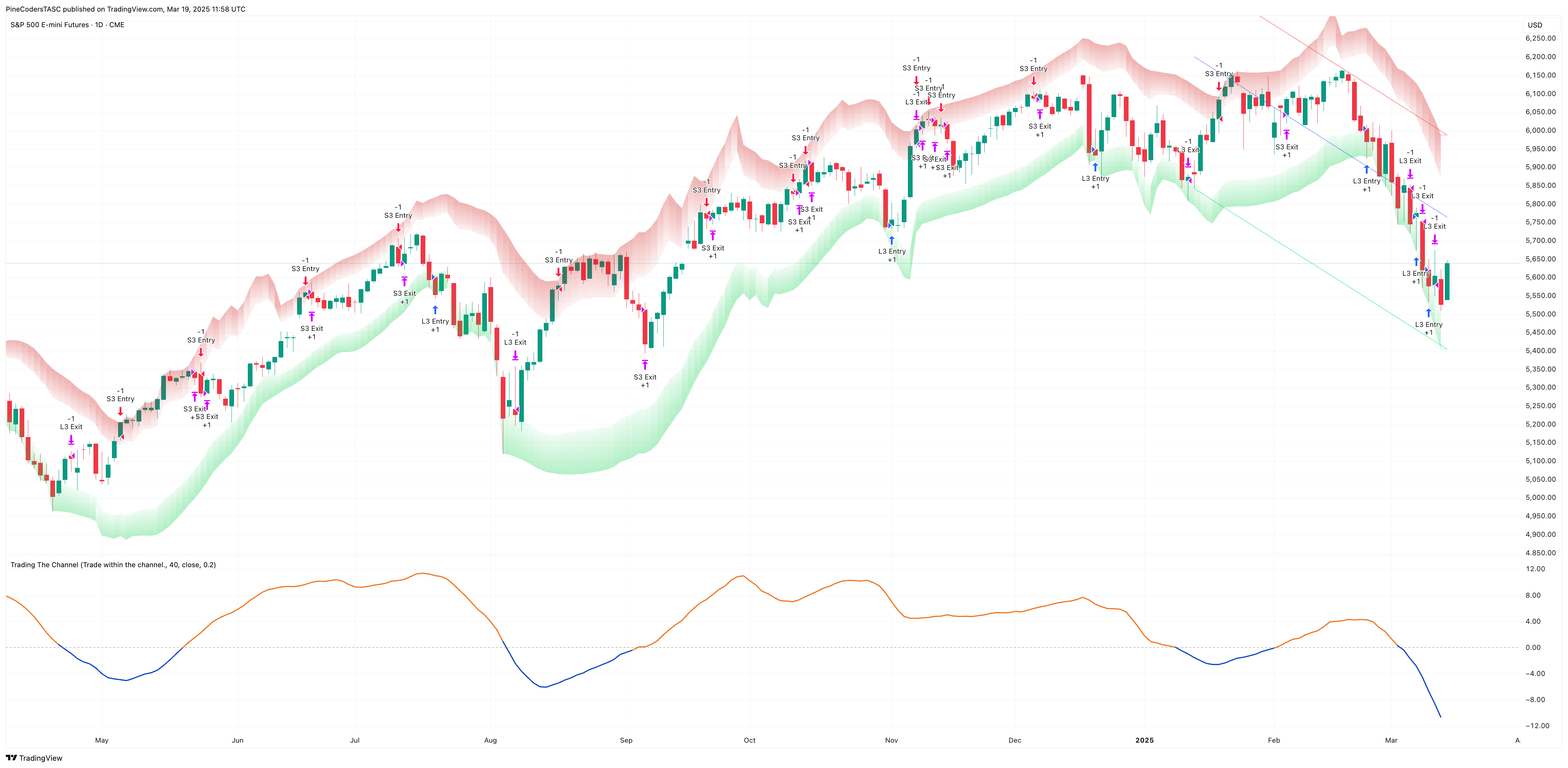
An example chart is shown in Figure 4.

FIGURE 4: TRADINGVIEW. This shows an example implementation of channel-based trading on a daily chart of the emini S&P 500 continuous futures contract.
—PineCoders, for TradingView
www.TradingView.com
BACK TO LIST

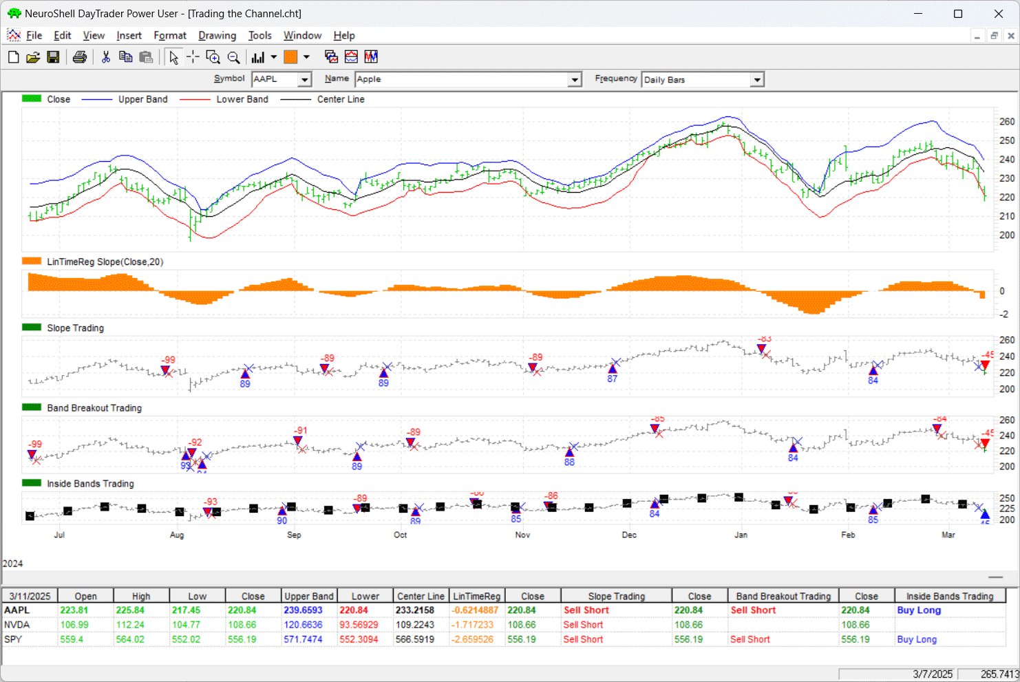
NeuroShell Trader: May 2025
The linear regression slope and upper/lower band trading systems discussed in Perry Kaufman’s article in this issue, “Trading The Channel,” can be easily implemented in NeuroShell Trader by combining some of NeuroShell Trader’s over 800 indicators. To implement the linear regression slope and upper/lower bands, select “New indicator” from the insert menu and use the indicator wizard to create the following indicators:
Slope:	LinTimeReg Slope(Close,20)
Center:	LinTimeReg PredValue(Close,20,0)
Upper band:	Add2(Center Line, Max(Sub(Close, Center Line),20))
Lower band:	Add2(Center Line, Min(Sub(Center Line),20))
To implement the slope and channel trading systems, select “New strategy” from the insert menu and use the trading strategy wizard to create the following three strategies:
Slope Trading System:
BUY LONG CONDITIONS:
     A>B(Slope, 0)
SELL SHORT CONDITIONS:
     A<B(Slope, 0)

Band Breakout Trading System:
BUY LONG CONDITIONS:
     A>B(High, Upper Band)
SELL SHORT CONDITIONS:
     A<B(Low, Lower Band)

	Inside Bands Trading System:
BUY LONG CONDITIONS:
     A<B(Close, Add2(Lower Band,Mul2(0.2,Sub(Upper Band, Lower Band))))
SELL SHORT CONDITIONS:
     A>B(Close, Sub(Upper Band, Mul2(0.2,Sub(Upper Band, Lower Band))))
Users of NeuroShell Trader can go to the Stocks & Commodities section of the NeuroShell Trader free technical support website to download a copy of this or any previous Traders’ Tips.

FIGURE 5: NEUROSHELL TRADER. This NeuroShell Trader chart demonstrates the different linear regression slope and band trading systems on a daily chart of AAPL.
—Ward Systems Group, Inc.
sales@wardsystems.com
www.neuroshell.com
BACK TO LIST

The Zorro Project: May 2025
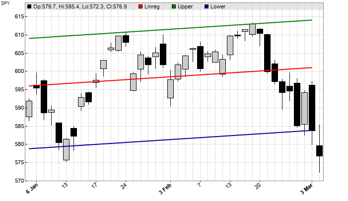
The simplest form of trend trading opens positions when the price crosses its moving average. In this issue, Perry Kaufman, in his article “Trading The Channel,” suggests an alternative using a linear regression line with an upper and lower band. Such a band indicator can be used to trigger long or short positions when the price crosses the upper or lower band, or when it gets close.
Let’s first code the bands. They have the same slope as the regression line and move through the highest and lowest price deviations from that line. Here’s the piece of code in C:
var Slope = LinearRegSlope(seriesC(),N);
var Intercept = LinearRegIntercept(seriesC(),N);
var LinVal, HighDev = 0, LowDev = 0;
for(i=N; i>0; i--) {
  LinVal = Intercept + Slope*(N-i);
  HighDev = max(HighDev,priceC(i)-LinVal);
  LowDev = min(LowDev,priceC(i)-LinVal);
}
A regression line has the formula y = b + m*x, where b is the intercept and m the slope. The code generates both for the previous N bars, then calculates in the loop the maximum and minimum deviations (HighDev, LowDev). The regression value (LinVal) is calculated from the intercept and slope with the above formula. Since the bar offset i runs backwards from the current bar, the bar number that’s multiplied with the slope runs from N down to 0.
Figure 6 shows an example result when the code is applied to a chart of SPY from 2025.

FIGURE 6: ZORRO. Here is an example of the regression line calculated and plotted on a daily chart of SPY for a portion of 2025, along with an upper and lower trading band. The regression value is calculated from the intercept and slope.
The candles can exceed the upper and lower bands because only the close price is used for them. It would probably improve the system, at least in theory, if we used the high and low prices instead.
Kaufman suggests several methods of trading with these bands; here, we’re using the “inside channel” method since it tends to be, according to Kaufman, the most profitable. We open a long position when the price comes within a zone around the lower band, and we close the position (or open a short position) when the price comes within a zone around the upper band.
Here is the trading system in C for Zorro, using the above code to calculate the bands:
void run()
{
  BarPeriod = 1440;
  StartDate = 20100101;
  LookBack = 150;
  assetList("AssetsIB");
  asset("SPY");
  if(is(LOOKBACK)) return;

  int i, N = 40;
  var Factor = 0.2;
  var Slope = LinearRegSlope(seriesC(),N);
  var Intercept = LinearRegIntercept(seriesC(),N);
  var LinVal, HighDev = 0, LowDev = 0;
  for(i=N; i>0; i--) {
    LinVal = Intercept + Slope*(N-i);
    HighDev = max(HighDev,priceC(i)-LinVal);
    LowDev = min(LowDev,priceC(i)-LinVal);
  }
  var Zone = Factor*(HighDev+LowDev);
  if(!NumOpenLong && priceC(0) < LinVal+LowDev+Zone)
    enterLong();
  if(!NumOpenShort && priceC(0) > LinVal+HighDev-Zone)
    exitLong();
}
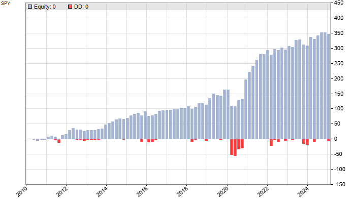
We’ve selected the AssetsIB asset list, which contains the margins, commissions, and other parameters from a U.S. brokerage. So the backtest simulates trading with that brokerage. The resulting equity curve with the default parameters, N = 40 and zone = 20%, already shows promise with a 2.8 profit factor (Figure 7.)

FIGURE 7: ZORRO. Here is an example equity curve from a backtest on data 2010–2024 plus a portion of 2025 to test a strategy based on trading inside the trading bands, where a long position is opened when price reaches or nears the lower band and exits when the price reaches or nears the upper band.
However, Kaufman mentions that he tested N values from 20 to 150, and zones from 5% to 50%. We’ll do the same by optimizing these parameters. Of course, a backtest with the best optimization result would be meaningless due to bias (see https://zorro-project.com/backtest.php). Therefore, we’re using walk-forward optimization for an out-of-sample backtest. Since anything with Zorro is done in code, we’ll insert some C code for the optimization:
set(PARAMETERS);
NumWFOCycles = 5;
N = optimize(40,20,150,10);
Factor = optimize(0.2,0.05,0.5,0.05);
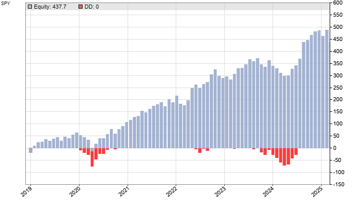
We also changed the trading from only long positions to both long and short by replacing exitLong with enterShort. By default, entering a short position automatically exits the long one, and vice versa. So the system is always in the market with 1 share, either long or short. The walk-forward optimization takes about 3 seconds. A resulting equity curve is shown in Figure 8. The profit factor rose to 7, with a 76% win rate.

FIGURE 8: ZORRO. Here is an example equity curve from a backtest of the same inside channel trading strategy as in Figure 7, this time with the N parameter optimized using walk-forward, out-of-sample optimization. The profit factor here is higher.
The code provided here can be downloaded from the 2025 script repository on https://financial-hacker.com. The Zorro platform can be downloaded from https://zorro-project.com.
—Petra Volkova
The Zorro Project by oP group Germany
https://zorro-project.com
BACK TO LIST

AIQ: May 2025
AIQ code based on Perry Kaufman’s article in this issue, “Trading The Channel,” is shown here and also provided in a downloadable code file. This encodes the system that the author describes as a linear regression slope trading system, which goes long when the linear regression slope goes above the zero line and exits when the linear regression slope drops below the zero line.
! TRADING THE CHANNEL
! Author: Perry J Kaufman, TASC May 2025
! Coded by: Richard Denning, 3/15/2025

! Example of trading the linear regression slope:
Len is 20.
C is [close].
LRslope is Slope2(C,Len).
Signal is iff(LRslope > 0,1,-1).

Buy if Signal = 1 and valresult(Signal,1) = -1.
ExitLong if Signal = -1.
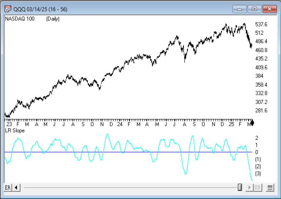
Figure 9 shows an example of the linear regression slope line plotted on a daily chart of QQQ (Nasdaq-100 ETF).

FIGURE 9: AIQ. The linear regression slope indicator is displayed on a daily chart of the Nasdaq-100 ETF (QQQ) during 2024 and into the first part of 2025.
—Richard Denning
rdencpa@gmail.com
for AIQ Systems
BACK TO LIST
Python: May 2025
Here, I am presenting some Python code to implement some of the concepts described in Perry Kaufman’s article in this issue, “Trading The Channel.” In the article, Kaufman discusses three approaches to trading with trading bands and also a linear regression line. Python programming language can be used to calculate and plot these elements on a chosen ticker symbol, and here, I will combine the calculations into one callable function after demonstrating the steps.
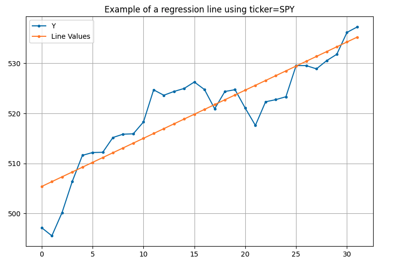
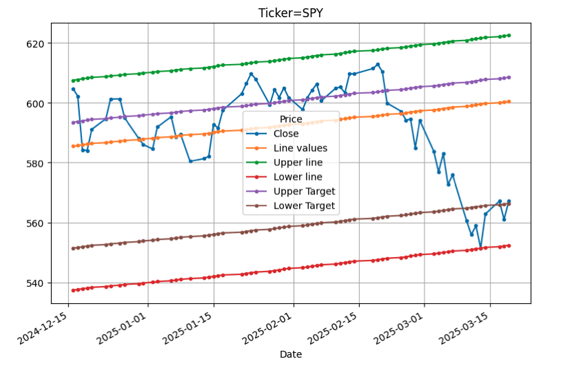
Figure 10 shows an example of plotting a regression line using Python, and Figure 11 shows an example of plotting trading bands with the regression line and target lines.

FIGURE 10: PYTHON. A linear regression line is plotted on a chart of SPY by using the built-in plotting function from the Panda data analysis library. The linear regression line is calculated from slope and y-intercept values calculated by the Python coding.

FIGURE 11: PYTHON. The upper and lower trading band lines, the upper and lower target lines, the linear regression line, and closing price line are plotted on a chart of SPY using calculations from a single callable function.
#
# import required python libraries
#
%matplotlib inline
import pandas as pd
import numpy as np
import matplotlib as mpl
import matplotlib.pyplot as plt
import yfinance as yf
import math
import datetime as dt

#
# Retrieve SPY daily price data from Yahoo Finance
#
#symbol = '^GSPC'
symbol = 'SPY'
end = dt.datetime.now().strftime('%Y-%m-%d')
ohlcv = yf.download(symbol, start="2019-01-01", end="2025-03-20", group_by="Ticker", auto_adjust=True)
ohlcv = ohlcv[symbol]

#
# Use pandas built in plot function to see simple price chart
#
ax = ohlcv['Close'].plot(
    figsize=(9,6),
    grid=True,
    title=f'{symbol}',
    #marker='.')

#
# the following python code snippets include the various calculation used to build the
# linear regression line
#

# use slicing techiques to extract desired set of close values based on end date and
# the linear regression window (aka _num_samples)
end_date = '2024-06-13'
num_samples = 32
samples = ohlcv['Close'][:end_date][-num_samples:].values.round(4)

# create x_values to corresend with num_samples
x_values = np.arange(len(samples))+1

# use numpy's polyfit to obtain slope, and y intercept
m, b = np.polyfit(x_values, samples, 1)

print(f'Slope={m}, Y-intercept={b}')

# calculate regression line values using m and b
line_values = m*x_values + b

# load the dataframe with desired values
df = pd.DataFrame()
df['X'] = x_values
df['Y'] = samples
df['Line Values'] = line_values
df

#
# Plot closing price and the linear regression line using built-in pandas plot
# function (aka using MatplotLib)
#
def simple_plot1(df):

    cols = ['Y', 'Line Values']
    ax = df[cols].plot(
        figsize=(9,6),
        grid=True,
        marker='.',
        title=f'Example of a regression line using ticker={symbol}'
    )

simple_plot1(df)

#
# combine all calculation from article into a single callable function
#
def run_daily_calculations(ohlcv, period, zone, verbose=False):

    df = ohlcv[-period:][['Close']].copy()
    # create x_values to corresend with num_samples
    x_values = np.arange(len(df))+1
    samples = df['Close'].values

    # use numpy's polyfit to obtain slope, and y intercept
    m, b = np.polyfit(x_values, samples, 1)

    if verbose:
        print(f'Slope={m}, Y-intercept={b}')

    df['X'] = x_values
    df['Slope'] = m
    df['Y-intercept'] = b
    df['Line values'] = m*x_values + b

    # calculations for upper and lower channels as per article
    df['Diff'] = df['Close'] - df['Line values']
    df['Upper line'] = df['Line values'] + df['Diff'][:-1].max()
    df['Lower line'] = df['Line values'] + df['Diff'][:-1].min()

    # calculations for upper and lower price targets as per article
    df['Upper Target'] = df['Upper line'] - zone *(df['Upper line']-df['Lower line'])
    df['Lower Target'] = df['Lower line'] + zone *(df['Upper line']-df['Lower line'])

    return df

def simple_plot2(df, usedates=False):

    import matplotlib.pyplot as plt

    if usedates is not True:
        df.set_index('X', inplace=True)

    cols = ['Close', 'Line values', 'Upper line', 'Lower line', 'Upper Target', 'Lower Target']
    ax = df[cols].plot(
        figsize=(9,6),
        grid=True,
        marker='.',
        title=f'Ticker={symbol}'
    )

##
# change the input parameters as desired and inspect resulting plot. The lines presented are
# calculated # based on the period. Inspect the far right of the plots (aka end_date) to look for
# price action to match your signal requirements.
#

#-------- INPUT PARAMETERS -------------
end_date = '2025'
period = 140
zone = 0.20
num_days_to_plot = 63
#---------------------------------------

df = run_daily_calculations(ohlcv[:], period, zone)
simple_plot2(df[-num_days_to_plot:], usedates=True)
—Rajeev Jain, jainraje@yahoo.com
BACK TO LIST
Microsoft Excel: May 2025
Perry Kaufman, in his article in this issue, “Trading The Channel,” describes three different trading rule sets that are based on the instantaneous slope and band width calculated for each bar, as has been done for the right-most bar in Figure 12. Playing with the values in cell A11 and/or cell A23 will demonstrate the dynamics of this computation.

FIGURE 12: EXCEL. Perry Kaufman’s article in this issue discusses channel-based trading methods based on the instantaneous slope and band width calculated for each bar. You see here the 30-bar best fine line through the right-most bar. The two touch points mark the close that is the farthest above and below the line and establish the upper and lower channel lines.
In Figure 13, the lower chart tracks the slope calculated in this way for each bar and assigns a plus or minus “trend” for a positive or negative slope. Figure 2 also displays the local results for long trades using the author’s rule 1, which only trades when the trend is positive. You may also select for a display of short trades.

FIGURE 13: EXCEL. The lower chart tracks the slope for each bar and assigns a plus or minus “trend” for a positive or negative slope. Local results are displayed for long trades using the author’s first rule set, which only trades when the trend is positive. (You can also use this spreadsheet to display short trades.) The blue X marks the close price that begins and ends a trade. Green is a winning trade, red is a losing trade.
Figure 14 plots the bar-by-bar calculated upper and lower band values (orange), and the percentage-of-spread zone values (green). The touch point mess occurs when a bar close meets or exceeds, in the rule 3 case, the bar zone value. A bar touch point, combined with the bar trend, determines the beginning and end of a long or short trade.

FIGURE 14: EXCEL. This example chart using NVDA plots the bar-by-bar calculated upper and lower band values (orange) and the percentage-of-spread zone values (green). When the bar close meets or exceeds the zones, a touch point is potentially triggered, in the case of one of the possible rule sets given by the article’s author.
Rule 2 uses touches of the bands (orange) instead of touches of the zones (green).
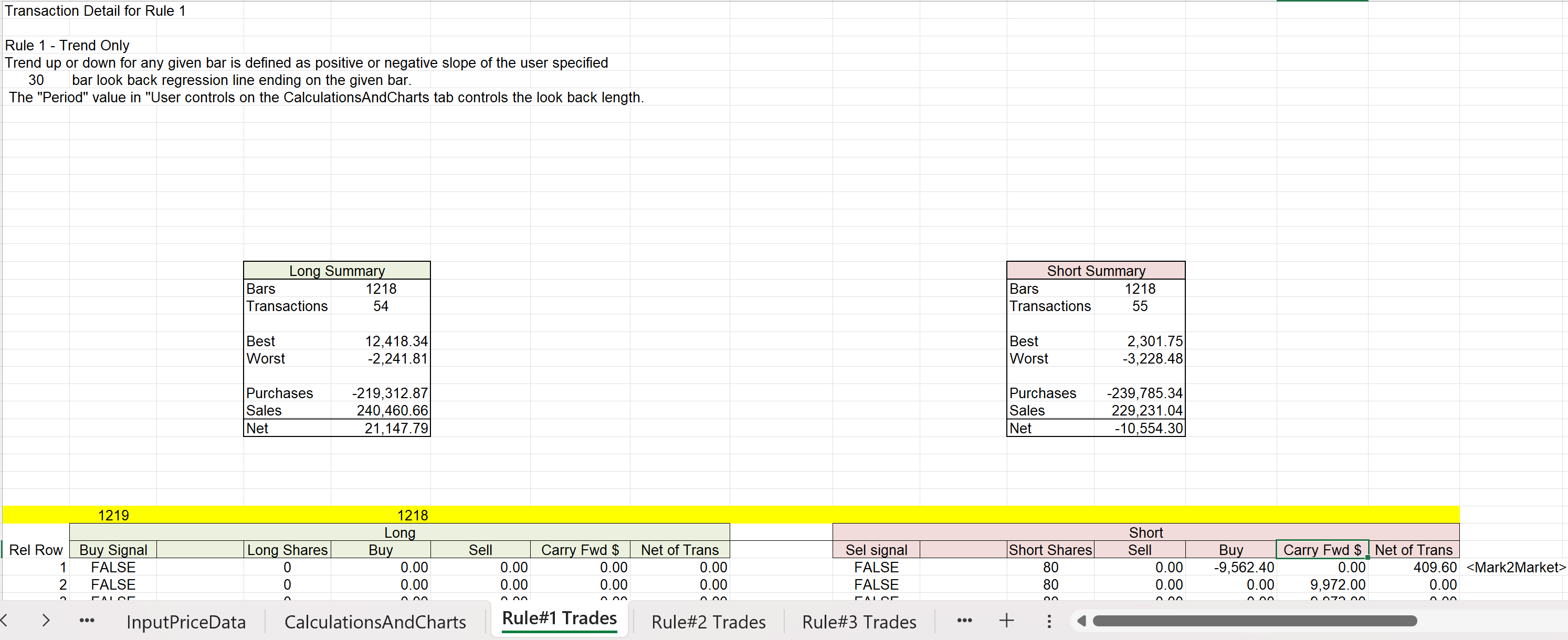
Figure 15 shows some trading results for rule 1. While Kaufman did not include short trades for stocks in his article, I went ahead and added shorts, based on his use of futures shorts, as a separate set of columns, as a test. In my small window of testing time, I can see why he did not include the shorts. Under these three rule sets, shorts appear to consistently lose money.

FIGURE 15: EXCEL. Here you see some example results from the trading rule in Figure 3. In the spreadsheet, each of the author’s three rule sets gets its own trade computations page with a results summary block for long and short trades. Values from these “rules” pages are pulled in to build the chart using the button combinations next to the charts.
Note: This month’s spreadsheet is a busy one! There will be a lot of computing involved if you change something and there is a lot of stuff hidden in the charts that only shows up when you select the correct combinations of “charting options” and “display of trades” using the buttons located to the right of the charts. Consequently, the spreadsheet and the charts will be a bit slow to react.
P.S. This spreadsheet also contains an updated repairs mechanism. See the “Traders Tips Repairs” tab in the spreadsheet for details.
To download this spreadsheet: The spreadsheet file for this Traders’ Tip can be downloaded here. To successfully download it, follow these steps:
- Right-click on the Excel file link, then
- Select “save as” (or “save target as”) to place a copy of the spreadsheet file on your hard drive.
—Ron McAllister
Excel and VBA programmer
rpmac_xltt@sprynet.com
BACK TO LIST
Originally published in the May 2025 issue of
Technical Analysis of STOCKS & COMMODITIES magazine.
All rights reserved. © Copyright 2025, Technical Analysis, Inc.


