TRADERS’ TIPS
March 2025

For this month’s Traders’ Tips, the focus is John F. Ehlers’ article in this issue, “Removing Moving Average Lag.” Here, we present the March 2025 Traders’ Tips code with possible implementations in various software.
You can right-click on any chart to open it in a new tab or window and view it at it’s originally supplied size, often much larger than the version printed in the magazine.
The Traders’ Tips section is provided to help the reader implement a selected technique from an article in this issue or another recent issue. The entries here are contributed by software developers or programmers for software that is capable of customization.

TradeStation: March 2025
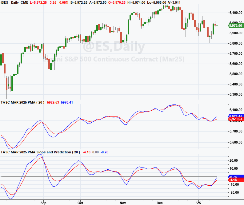
In “Removing Moving Average Lag” in this issue, John Ehlers introduces a projected moving average (PMA) designed to remove the lag inherent in moving averages. He does this by adding the slope times half the length of the average to the average itself. A function labeled $PMA is provided for the calculations. A sample chart displaying the PMA, the PMA slope, and its prediction, as discussed in Ehlers’ article, is shown in Figure 1.

FIGURE 1: TRADESTATION. A daily chart of the continuous emini S&P 500 (ES) showing a portion of 2024 and 2025 with the two indicators applied, the projected moving average and the slope, using a length of 20.
Function: $PMA
{
	TASC MAR 2025
	Projected Moving Average ($PMA) Function
	(C) 2024 John F. Ehlers
}

inputs:
	Price( numericseries ),
	Length( numericsimple ),
	PMA( numericref ),
	Slope( numericref ),
	SMA( numericref );

variables:
	Count( 0 ),
	Sx( 0 ),
	Sy( 0 ),
	Sxx( 0 ),
	Syy( 0 ),
	Sxy( 0 );

Sx = 0;
Sy = 0;
Sxx = 0;
Syy = 0;
Sxy = 0;

for Count = 1 to Length
begin
	Sx = Sx + Count;
	Sy = Sy + Price[Count - 1];
	Sxx = Sxx + Count * Count;
	Syy = Syy + Price[Count - 1] * Price[Count - 1];
	Sxy = Sxy + count*Price[Count - 1];
end;

Slope = -(Length * Sxy - Sx * Sy) / (Length * Sxx - Sx * Sx);
SMA = Sy / Length;
PMA = SMA + Slope * Length / 2;

//Function Return Value
$PMA = 1;


Indicator: Projected Moving Average (PMA)
{
	TASC MAR 2025
	Projected Moving Average (PMA)
	(C) 2024 John F. Ehlers
}

inputs:
	Length( 20 );

variables:
	ReturnValue( 0 ),
	PMA( 0 ),
	Slope( 0 ),
	SMA( 0 ),
	Predict( 0 );

ReturnValue = $PMA(Close, Length, PMA, Slope, SMA);
Predict = PMA + .5 * (Slope - Slope[2])*Length;

Plot1( PMA, "PMA" );
Plot2( Predict, "Predict" );
//Plot3( SMA, "SMA" )


Indicator: PMA Slope and Prediction
{
	TASC MAR 2025
	PMA Slope and Its Prediction
	(C) 2024 John F. Ehlers
}

inputs:
	Length( 20 );

variables:
	ReturnValue( 0 ),
	PMA( 0 ),
	Slope( 0 ),
	SMA( 0 ),
	Predict( 0 );

ReturnValue = $PMA(Close, Length, PMA, Slope, SMA);
Predict = 1.5 * Slope - .5 * Slope[4];

Plot1( Slope, "Slope" );
Plot2( 0, "Zero Line" );
Plot3( Predict, "Predict" );
This article is for informational purposes. No type of trading or investment recommendation, advice, or strategy is being made, given, or in any manner provided by TradeStation Securities or its affiliates.
—John Robinson
TradeStation Securities, Inc.
www.TradeStation.com
BACK TO LIST

Wealth-Lab.com: March 2025
We have implemented John Ehlers’ projected moving average (PMA) as a core indicator that comes out of the box in WealthLab 8.
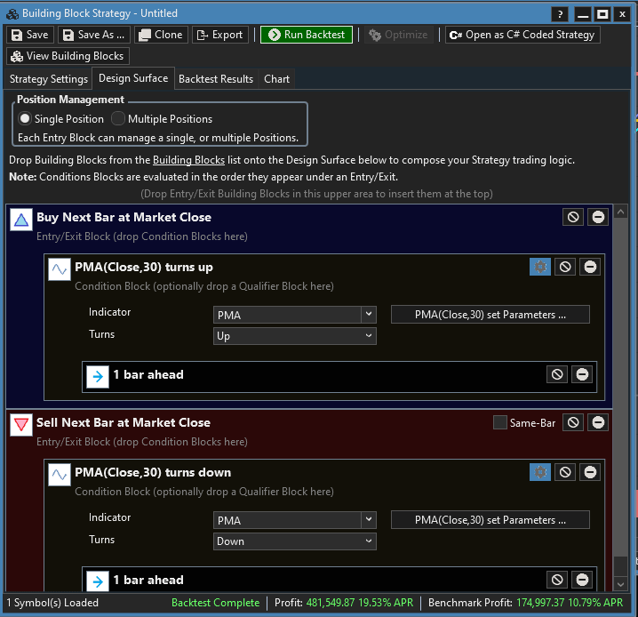
We can put it to the test with a simple strategy created with drag-and-drop building blocks (Figure 2). We enter at market close when the PMA(30) turns up and exit at market close when it turns down. WealthLab 8’s Strategy Monitor has built-in features to allow you to trade an “at-close” strategy like this by running it a few seconds before the actual close and using the up-to-the-second closing price as a proxy for the eventual actual close. In a test on TQQQ, this simple example strategy generated an annualized return of nearly 20% with and average profit of 1.69% per trade.

FIGURE 2: WEALTH-LAB. With the Building Blocks feature in Wealth-Lab, the user can build a strategy to test using drag-and-drop. Here, an example strategy is creating incorporating John Ehlers’ projected moving average as a prebuilt indicator.
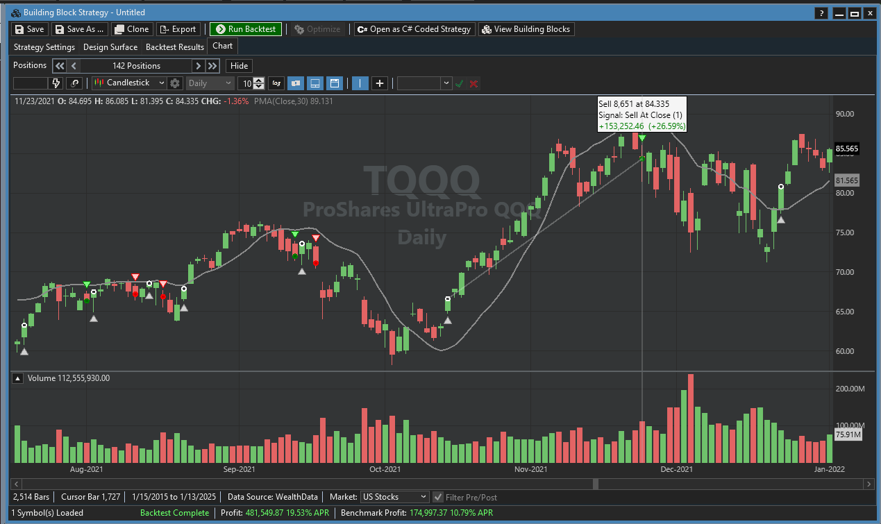
An example chart showing the PMA along with the example strategy on a chart of TQQQ is in Figure 3.

FIGURE 3: WEALTH-LAB. Here you see the projected moving average (PMA) and an example buy/sell strategy on a daily chart of TQQQ.
—Dion Kurczek
Wealth-Lab team
www.wealth-lab.com
BACK TO LIST

TradingView: March 2025
Here is TradingView Pine Script code implementing John Ehlers’ projected moving average (PMA), introduced in his article in this issue titled “Removing Moving Average Lag.” The PMA is designed to remove the lag inherent in moving averages.
//  TASC Issue: March 2025
//     Article: A New Solution
//              Removing Moving Average Lag
//  Article By: John F. Elhers
//    Language: TradingView's Pine Script® v6
// Provided By: PineCoders, for tradingview.com

//@version=6
title ='TASC 2025.03 A New Solution'+
     ' Removing Moving Average Lag'
stitle = 'TASC'
indicator(title, stitle, false)

// @function Projected Moving Average.
// @param src Source series.
// @param length Length.
// @returns
// - `PMA` Projected Moving Average.
// - `SMA` Simple Moving Average.
// - `Slope` Calculated Slope.
pma (float src, int length) =>
    float Sx = 0.0 , float Sy = 0.0
    float Sxx = 0.0 , float Syy = 0.0 , float Sxy = 0.0
    for count = 1 to length
        float src1 = src[count - 1]
        Sx += count
        Sy += src[count - 1]
        Sxx += count * count
        Syy += src1 * src1
        Sxy += count * src1
    float Slope = -(length*Sxy-Sx*Sy) / (length*Sxx-Sx*Sx)
    float SMA = Sy / length
    float PMA = SMA + Slope * length / 2
    [PMA, SMA, Slope]

//#endregion

// @enum Display mode fields:
// @field MA Display moving averages.
// @field SP Display Slope and Prediction.
enum DISP
    MA = 'Moving Averages'
    SP = 'Slope And Prediction'

DISP disp = input.enum(DISP.MA, 'Display Mode:')
float src = input.source(close, 'Source:')
int length = input.int(30, 'Length:')

bool is_disp_ma = disp == DISP.MA
bool is_disp_sp = disp == DISP.SP

[pma, sma, slope] = pma(src, length)
float predict = switch
    is_disp_ma => pma + .5 * (slope - slope[2]) * length
    is_disp_sp => 1.5 * slope - 0.5 * slope[4]
    => float(na)

show_ma = is_disp_ma ? display.all : display.none
show_sp = is_disp_sp ? display.all : display.none

plot(src, 'SRC', color.blue, display=show_ma)
plot(pma, 'PMA', color.green, display=show_ma)
plot(predict, 'Predict', color.lime, display=show_ma)
plot(sma, 'SMA', color.red, display=show_ma)

plot(slope, 'Slope', color.blue, display=show_sp)
plot(0, '0', color.silver, display=show_sp)
plot(predict, 'Predict', color.lime, display=show_sp)
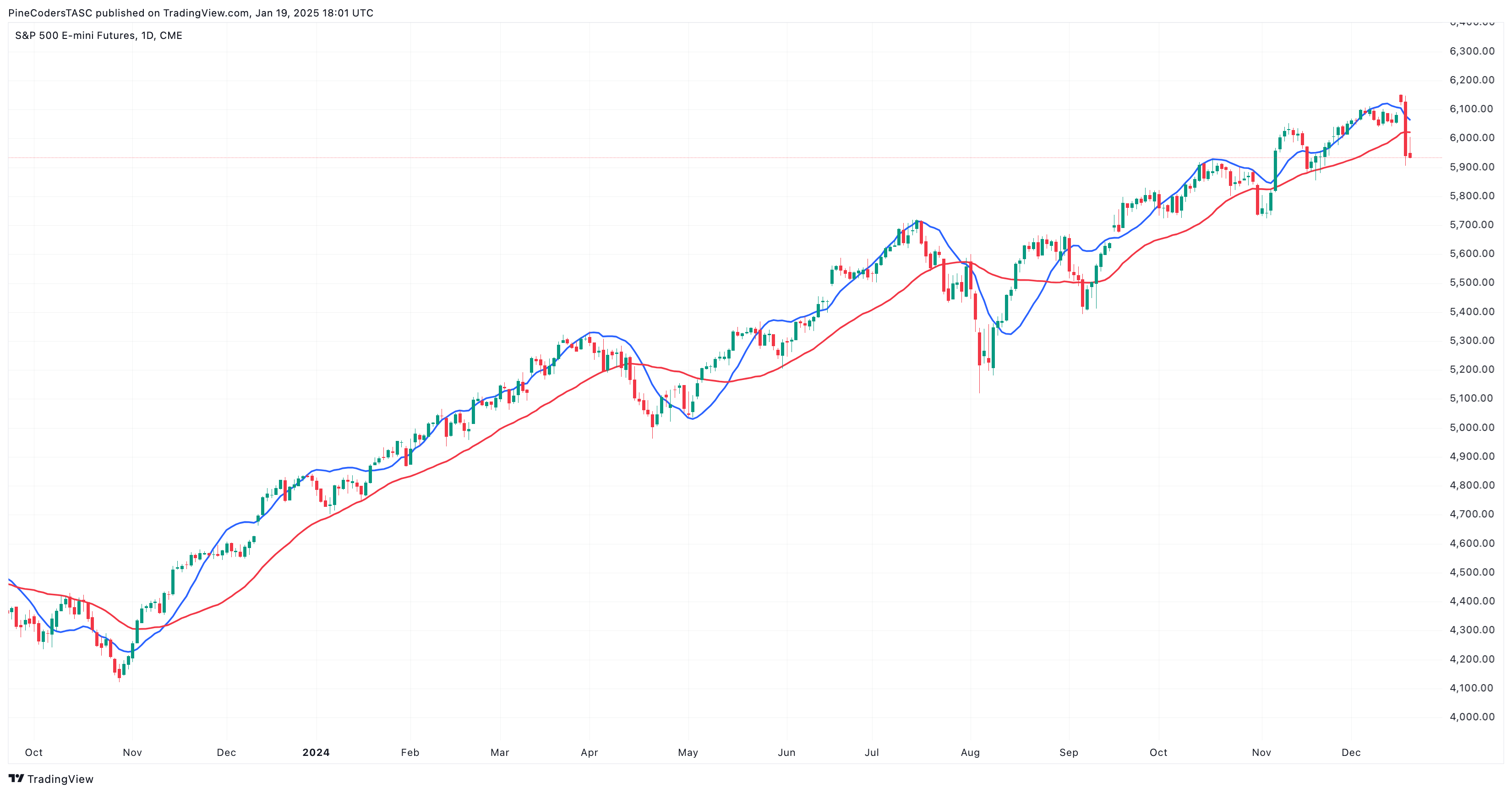
An example chart displaying the PMA is shown in Figure 4.

FIGURE 4: TRADINGVIEW. This displays the projected moving average (PMA) on a daily chart of the emini S&P futures contract (ES).
The indicator is available on TradingView from the PineCodersTASC account: https://www.tradingview.com/u/PineCodersTASC/#published-scripts.
—PineCoders, for TradingView
www.TradingView.com
BACK TO LIST

Neuroshell Trader: March 2025
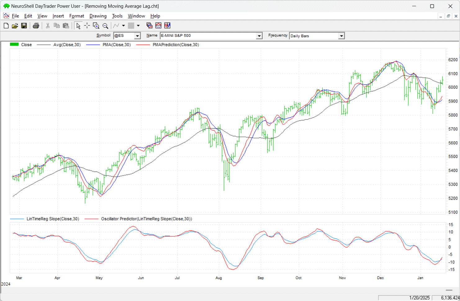
The projected moving average, its prediction, the slope oscillator, and the oscillator prediction, described in John Ehlers’ article in this issue titled “Removing Moving Average Lag,” can be easily implemented in NeuroShell Trader by selecting “New indicator ...” from the insert menu and using the indicator wizard to create the following indicators:
Slope:	LinTimeReg Slope(Close,30)
PMA:	Add2(Avg(Close,30),Mul3(Slope, 30,0.5))

PMA Prediction:	Add2(PMA,Mul3(0.5,Momentum(Slope,2),30))

Oscillator Prediction:	Sub(Mul2(1.5, Oscillator),Mul2(0.5,Lag(Oscillator, 4)))

FIGURE 5: NEUROSHELL TRADER. This NeuroShell Trader chart shows a moving average, the projected moving average (PMA), PMA prediction, slope oscillator, and the slope oscillator prediction on a daily chart of the emini S&P 500 futures contract (ES).
Users of NeuroShell Trader can go to the Stocks & Commodities section of the NeuroShell Trader free technical support website to download a copy of this or any previous Traders’ Tips.
—Ward Systems Group, Inc.
sales@wardsystems.com
www.neuroshell.com
BACK TO LIST

RealTest: March 2025
Provided here is coding for use in the RealTest platform to implement the indicators described in John Ehlers’ article in this issue, “Removing Moving Average Lag.”
Notes:
	Projected Moving Average
	TASC Trader's Tips for March 2025 article by John Ehlers

Import:
	DataSource:	Norgate
	IncludeList:	&ES
	StartDate:	1/1/20
	EndDate:	Latest
	SaveAs:	es.rtd

Settings:
	DataFile:	es.rtd
	StartDate:	Earliest
	EndDate:	Latest
	BarSize:	Daily

Parameters:
	len:	20

Data:
	smaN:	avg(c, len)
	slopeN:	slope(c, len)
	pmaN:	smaN + slopeN * len / 2
	pmaPredict:	pmaN + 0.5 * (slopeN - slopeN[2]) * len
	slopePredict:	1.5*slopeN-0.5*slopeN[4]

Charts:
	smaN:	smaN
	pmaN:	pmaN
	pmaPredict:	pmaPredict
	slopeN:	slopeN {|}
	slopePredict:	slopePredict {|}
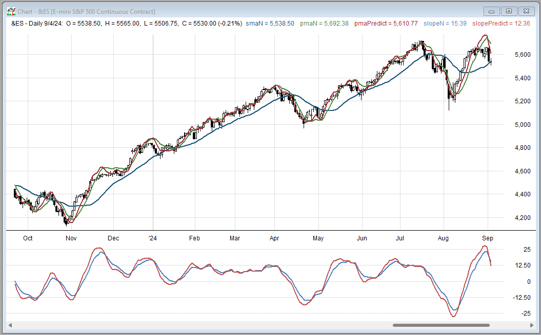
Figure 6 shows an example of the projected moving average on a daily chart of the emini S&P futures contract (ES).

FIGURE 6: REALTEST. Here you see an example of John Ehlers’ projected moving average (PMA) on a daily chart of the emini S&P 500 (ES).
—Marsten Parker
MHP Trading
mhp@mhptrading.com
BACK TO LIST

The Zorro Project: March 2025
In his article in this issue, “Removing Moving Average Lag,” John Ehlers proposes a moving average variant that does not suffer from the usual moving average problem: lag. A simple moving average lags by half its period behind the price. The projected moving average (PMA) indicator overcomes this problem by projecting its value by half a period into the future—thus, zero lag.
The PMA function provided here is a straightforward conversion to C of Ehlers’ EasyLanguage code given in his article in this issue.
var PMA(vars Data,int Length)
{
  var Sx = 0, Sy = 0, Sxx = 0, Syy = 0, Sxy = 0;
  int i;
  for(i=1; i<=Length; i++) {
    Sx += i;
    Sy += Data[i-1];
    Sxx += i*i;
    Syy += Data[i-1]*Data[i-1];
    Sxy += i*Data[i-1];
  }
  var Slope = -(Length*Sxy - Sx*Sy) / (Length*Sxx - Sx*Sx);
  return Sy/Length + Slope*Length/2;
}
The Sy/Length term in the above function corresponds to a standard moving average. For comparing the PMA with an SMA, we can apply both to an SPX chart from 2024, using the following code:
void run()
{
  BarPeriod = 1440;
  StartDate = 20231001;
  EndDate = 20241001;
  LookBack = 30;
  assetAdd("SPX","STOOQ:^SPX");
  asset("SPX");
  plot("PMA",PMA(seriesC(),LookBack),LINE,BLUE);
  plot("SMA",SMA(seriesC(),LookBack),LINE,RED);
}

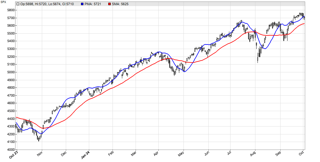
FIGURE 7: ZORRO. This example chart of the daily ES displays the projected moving average (PMA) in blue, and a simple moving average (SMA) is in red for comparison.
We can see that the PMA (blue) follows the price line much closer than the SMA (red) with the same period.
The code can be downloaded from the 2025 script repository on https://financial-hacker.com. The Zorro platform can be downloaded from https://zorro-project.com.
—Petra Volkova
The Zorro Project by oP group Germany
https://zorro-project.com
BACK TO LIST

NinjaTrader: March 2025
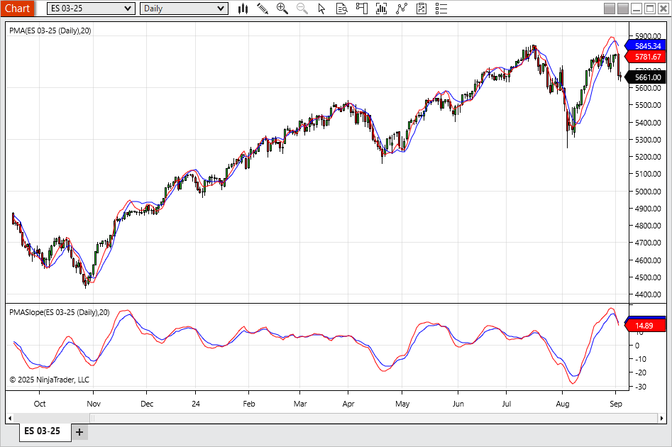
In “Removing Moving Average Lag” in this issue, John Ehlers presents the projected moving average (PMA) and some accompanying indicators. Several of the indicators discussed in the article are available for download at the following link for NinjaTrader 8:
Once the file is downloaded, you can import the indicator into NinjaTrader 8 from within the control center by selecting Tools → Import → NinjaScript Add-On and then selecting the downloaded file for NinjaTrader 8.
You can review the indicator source code in NinjaTrader 8 by selecting the menu New → NinjaScript Editor → Indicators folder from within the control center window and selecting the file.
A sample chart is shown in Figure 8.

FIGURE 8: NINJATRADER. The PMA and slope indicators are demonstrated on a daily chart of ES.
NinjaScript uses compiled DLLs that run native, not interpreted, to provide you with the highest performance possible.
—Jesse N.
NinjaTrader, LLC
www.ninjatrader.com
BACK TO LIST
Python: March 2025
In “Removing Moving Average Lag” in this issue, John Ehlers introduces his projected moving average (PMA), designed to remove the lag inherent in moving averages. His approach involves adding the slope times half the length of the average to the average itself to accomplish the projected moving average. The code listings given in Ehlers’ article cover the projected moving average as a function; the projected moving average indicator (and its prediction) to plot on a chart; and slope and its prediction, which in this case is an output from the PMA function code and is used to create an oscillator.
Following is an implementation of Ehlers’ coding in Python:
#
# import required python libraries
#
import pandas as pd
import numpy as np
import datetime as dt

import matplotlib.pyplot as plt
import yfinance as yf


#
# Retrieve S&P 500 daily price data from Yahoo Finance
#

symbol = '^GSPC'
ohlcv = yf.download(symbol, start="2015-01-15", end="2025-01-22")
ohlcv


#
# Introducing the Projected Moving Average PMA
#

def linear_regression_slope(samples):
    # Use numpy's polyfit to calculate the slope (1st degree polynomial)
    m, b = np.polyfit(np.arange(len(samples)), np.array(samples), 1)

    return m

def calc_linear_regression_slope(in_series, length):
    slope = in_series.rolling(length).apply(linear_regression_slope)
    return slope

def calc_sma(in_series, length):
    return in_series.rolling(length).mean()

def calc_pma(in_series, length):
    sma = calc_sma(in_series, length)
    slope = calc_linear_regression_slope(in_series, length)
    pma = (sma + slope * length / 2)
    return pma


#
# S&P500 applying SMA and PMA indicators using 30 trading days
#

length = 30
df = ohlcv.copy()

df['SMA'] = calc_sma(df['Close'], length)
df['PMA'] = calc_pma(df['Close'], length)
simple_plot1(df['2023-09':'2024-09-04'], length)


#
# S&P500 applying SMA and PMA indicators using 200 trading days
#

length = 200
df = ohlcv.copy()

df['SMA'] = calc_sma(df['Close'], length)
df['PMA'] = calc_pma(df['Close'], length)
simple_plot1(df['2023-09':'2024-09-04'], length)


#
# Prediction to Further Reduce Lag
#

def calc_pma_prediction(pma, slope, length):
    # Predict = PMA + 0.5*(Slope - Slope[2])*Length
    predict = pma + (slope - slope.shift(2)) * length / 2

    return predict


#
# S&P500 applying PMA and PMA Prediction indicators
#


length = 30
df = ohlcv.copy()

df['SMA'] = calc_sma(df['Close'], length)
df['PMA'] = calc_pma(df['Close'], length)
#df['LRC'] = df['Close'].rolling(length).apply(linear_regression_curve)
df['Slope'] = df['Close'].rolling(length).apply(linear_regression_slope)
df['Predict'] = calc_pma_prediction(df['PMA'], df['Slope'], length)
df['Signal'] = np.where(df['Predict'] > df['PMA'], 1, 0)
simple_plot2(df['2023-09':'2024-09-04'], length, signal_ena=True)


#
# Introducing Generalized Prediction of an Indicator
#

def calc_general_prediction(smooth):

    predict = 1.5*smooth - 0.5*smooth.shift(4)
    return predict


#
# S&P 500 appling Slope and Slope Prediction indicators
#

length = 30
df = ohlcv.copy()

df['SMA'] = calc_sma(df['Close'], length)
df['PMA'] = calc_pma(df['Close'], length)

#df['LRC'] = df['Close'].rolling(length).apply(linear_regression_curve)
df['Slope'] = df['Close'].rolling(length).apply(linear_regression_slope)
df['Predict'] = calc_pma_prediction(df['PMA'], df['Slope'], length)
df['Slope Predict'] = calc_general_prediction(df['Slope'])
Figure 9 displays an example of a 30-day PMA on a daily chart of the S&P 500 index along with a 30-day simple moving average (SMA) for comparison. Figure 10 shows an example of the PMA and PMA prediction indicators. Figure 11 shows an example of plotting slope and its prediction.

FIGURE 9: PYTHON. This displays an example of a 30-day PMA on a daily chart of the S&P 500 index along with a 30-day simple moving average (SMA) for comparison. The projected moving average, introduced by John Ehlers in his article in this issue, was coded here using the Python language and then plotted using Matplotlib.

FIGURE 10: PYTHON. Here, the PMA and PMA prediction indicators are plotted on S&P 500 index daily data downloaded from Yahoo Finance. The vertical light-blue lines highlight the PMA and PMA prediction indicator crossovers.

FIGURE 11: PYTHON. Here, slope and its prediction are plotted.
—Rajeev Jain
jainraje@yahoo.com
BACK TO LIST
Python: February 2025
In the article “Drunkard’s Walk: Theory And Measurement By Autocorrelation” that appeared in the February 2025 issue, John Ehlers presents coding for his autocorrelation indicator and periodogram display, a technique Ehlers designed to help to analyze price data over different periods.
Following is an implemention of Ehlers’ autocorrelation indicator coding to the Python programming language. Figures 12–14 illustrate some of the steps carried out in the code.
# Generate 100 random variables in 5 batches of 20, between -1.0 and 1.0
import pandas as pd
import numpy as np
import random

def rand():
    return random.random()

random_values = []
for x in list(range(5)):
    for i in list(range(20)):
        random_values.append(2*(rand()-0.5))

x_values = np.arange(1, len(random_values) + 1)
df = pd.DataFrame(index=x_values, columns=['A'], data=random_values)
df

df['C'] = 0
df['D'] = 0

# Apply the formulas for first-order discrete random walk
# C[n] = 0.1 + C[n-1] + A[n]
for i in range(3, len(df)+1):
    df.loc[i, 'C'] = 0.1 + df.loc[i-1, 'C'] + df.loc[i, 'A']

# Apply the formulas for second-order discrete random walk
# D[n] = 0.1 + (D[n-1] + A[n-1] + A[n])/2
for i in range(3, len(df)+1):
    df.loc[i, 'D'] = 0.1 + (df.loc[i-1, 'D'] + df.loc[i-1, 'A'] + df.loc[i, 'A'])/2

df
# Plot results
df = df.rename(columns={'C':'1st Order','D':'2nd Order'})
cols = ['1st Order', '2nd Order']
ax = df[cols].plot(figsize=(9, 6), grid=True, title='First and Second Order Discrete Randowm Walk Simulations')

# Implement Ultimate Smoother Function
def ultimate_smoother(price_data, period):
    """
    Ultimate Smoother Function (as described by John Ehlers)

    Parameters:
    price_data (list or numpy array): The price series to smooth.
    period (int): The period used for the smoothing.

    Returns:
    numpy array: The smoothed price series.
    """

    # Initialize arrays to store the smoothed values and intermediate variables
    US = np.zeros_like(price_data)

    # Calculate the smoothing coefficients
    a1 = np.exp(-1.414 * 3.14159 / period)
    b1 = 2 * a1 * np.cos(1.414 * 180 / period)
    c2 = b1
    c3 = -a1 * a1
    c1 = (1 + c2 - c3) / 4

    # Apply the smoothing function (recursive filter)
    for i in range(len(price_data)):
        if i >= 2:  # Start applying the recursive formula after the 2nd index (CurrentBar >= 4)
            US[i] = (1 - c1) * price_data[i] + (2 * c1 - c2) * price_data[i - 1] \
                    - (c1 + c3) * price_data[i - 2] + c2 * US[i - 1] + c3 * US[i - 2]
        else:
            # For the first few points, just use the price value (no smoothing yet)
            US[i] = price_data[i]

    return US

# Plot UltimateSmoother using a 20-day period on S&P 500 closing data
import pandas as pd
import numpy as np
import matplotlib.pyplot as plt
import yfinance as yf

symbol = '^GSPC'
ohlcv = yf.download(symbol, start="2023-12-25", end="2024-12-25")

df = ohlcv.copy()
df['US/20'] = ultimate_smoother(prices=df['Close'], period=20)
cols = [
    'Close',
    'US/20',
]
ax = df[cols].plot(figsize=(12,8), grid=True, title=f"{symbol}, Ultimate Smoother / 20day period", marker='.')

# Autocorrelation indicator calculation
def autocorrelation_indicator(data, length=20):
    # Apply UltimateSmoother
    filt = ultimate_smoother(data, length)
    num_lags = 100  # Number of lags (0 to 99)
    num_bars = len(filt)  # Number of time points (bars)

    # Initialize the correlation matrix (2D array)
    corr_matrix = np.zeros((num_lags, num_bars))  # Shape: [lags, time]

    # Calculate correlation for each lag
    for lag in range(num_lags):
        for time_idx in range(length, num_bars):  # Start after smoothing length
            sx = sy = sxx = sxy = syy = 0
            for j in range(length):
                x = filt[time_idx - j] if (time_idx - j) >= 0 else 0
                y = filt[time_idx - lag - j] if (time_idx - lag - j) >= 0 else 0

                sx += x
                sy += y
                sxx += x * x
                sxy += x * y
                syy += y * y


            # Ensure the denominator is positive before calculating the correlation
            denominator_x = (length * sxx - sx ** 2)
            denominator_y = (length * syy - sy ** 2)

            if denominator_x > 0 and denominator_y > 0:
                corr_matrix[lag, time_idx] = (length * sxy - sx * sy) / sqrt(denominator_x * denominator_y)

    return corr_matrix

def plot_heatmap(corr_matrix):
    fig, ax = plt.subplots(figsize=(12, 6))  # Adjust figure size to make the plot clearer
    im = ax.imshow(corr_matrix, aspect='auto', interpolation='nearest', cmap='RdYlGn_r')  # Use a diverging colormap

    # Set axis labels
    ax.set_xlabel('Time (Index)', fontsize=12)
    ax.set_ylabel('Lag', fontsize=12)
    ax.set_title('AutoCorrelation Heatmap', fontsize=14)

    # Set ticks for lags (vertical axis)
    ax.set_yticks(np.arange(0, 100, 10))
    ax.set_yticklabels(np.arange(0, 100, 10))

    # Set ticks for time (horizontal axis)
    ax.set_xticks(np.arange(0, corr_matrix.shape[1], corr_matrix.shape[1] // 10))  # Ticks every ~10 bars
    ax.set_xticklabels(np.arange(0, corr_matrix.shape[1], corr_matrix.shape[1] // 10))

    # Add color bar
    cbar = fig.colorbar(im, ax=ax)
    cbar.set_label('Correlation Value', fontsize=12)

    plt.show()
price_data = ohlcv['Close'].tolist()

# Calculate the autocorrelation matrix
corr_matrix = autocorrelation_indicator(price_data, length=20)

# Plot the heatmap
plot_heatmap(corr_matrix)

FIGURE 12: PYTHON. Formulas are applied to create a first-order discrete random walk simulation and a second-order discrete random walk simulation. The plot is drawn using Matplotlib.

FIGURE 13: PYTHON. Here is an example of a 20-day UltimateSmoother indicator (orange) plotted on a daily chart of the S&P 500 stock index using data from Yahoo Finance (blue). The chart is created using Matplotlib.

FIGURE 14: PYTHON. A heatmap is plotted based on John Ehlers' autocorrelation indicator. The autocorrelation indicator uses Ehlers' UltimateSmoother indicator and calculates correlation for each lag.
—Rajeev Jain
jainraje@yahoo.com
BACK TO LIST
Originally published in the March 2025 issue of
Technical Analysis of STOCKS & COMMODITIES magazine.
All rights reserved. © Copyright 2025, Technical Analysis, Inc.
