TRADERS’ TIPS

April 2015

For this month’s Traders’ Tips, the focus is mainly Dave Cline’s article in this issue, “Basket Trading Using A Directed Acyclic Graph”, with some Traders’ Tips focusing on “Kiss & Touch With The Modified True Range” by Chris Lindgren, which appeared in the February 2015 issue. Here, we present the April 2015 Traders’ Tips code with possible implementations in various software.

Code already provided by Cline or Lindgren in their articles can be found in the Subscriber Area of our website here.

The Traders’ Tips section is provided to help the reader implement a selected technique from an article in this issue or another recent issue. The entries here are contributed by software developers or programmers for software that is capable of customization.

TRADESTATION: APRIL 2015
eSIGNAL: APRIL 2015
WEALTH-LAB: APRIL 2015
NEUROSHELL TRADER: APRIL 2015
AIQ: APRIL 2015
TRADERSSTUDIO: APRIL 2015
UPDATA: APRIL 2015
MICROSOFT EXCEL: APRIL 2015

TRADESTATION: APRIL 2015

In the February 2015 STOCKS & COMMODITIES article “Kiss & Touch With The Modified True Range,” author Chris Lindgren describes an indicator to help estimate the probability of an option’s underlying touching or reaching a certain price any time before expiration. Lindgren describes several ways that he uses the new indicator, which is itself is a modification to J. Welles Wilder’s true range.

For users’ convenience, we are providing EasyLanguage code for implementing the indicator in TradeStation.

Indicator: Modified True Range

inputs:
	Goal( 10 ),
	PeriodLength( 40 ) ;
	
variables:
	MTR( 0 ),
	AvgMTR( 0 ),
	StdDevMTR( 0 ),
	GoalCount( 0 ),
	GoalPctAchieved( 0 ),
	GoalAchieved( 0 ) ;
	
MTR = Maxlist( AbsValue( High - Close[1] ), 
	AbsValue( Low - Close[1] ) ) ;		

AvgMTR = Average( MTR, PeriodLength ) ; 

StdDevMTR = StdDev( MTR, PeriodLength ) ;

if  MTR >= Goal then
	begin
	GoalAchieved = 1 ;
	SetPlotColor( 10, Green ) ;
	end 
else
	begin
	GoalAchieved = 0 ; 
	SetPlotColor( 10, Red ) ;
	end ;

GoalCount = CountIf( GoalAchieved = 1, PeriodLength ) ;
GoalPctAchieved = iff( PeriodLength > 0, 100 
	* GoalCount / PeriodLength, 0 ) ;

//Status Line Plots
Plot1( "Goal Count : " + NumToStr ( GoalCount, 0 ) 
	+ Spaces( 5 ) , "Count", Yellow ) ;
Plot2( "Goal PCT : " + NumToStr ( GoalPctAchieved, 2 ) 
	+ "%" + Spaces( 5 ) , "CountPct", Yellow ) ;
Plot3( "Avg MTR : " + NumToStr ( AvgMTR, 2 ) 
	+ Spaces( 5 ) , "AVGMTR", Yellow ) ;
Plot4( "MTR Std Dev : " + NumToStr ( StdDevMTR, 2 ) 
	+ Spaces( 5 ) , "MTR Std Dev", Yellow ) ;

//Chart Plots
Plot10( MTR, "MTR" ) ;
Plot11( Goal, "Goal" ) ;

To download the EasyLanguage code, please visit our TradeStation and EasyLanguage support forum. The code from this article can be found here: https://www.tradestation.com/TASC-2015. The ELD filename is “_TASC_ModifiedTrueRange.ELD.” For more information about EasyLanguage in general, please see https://www.tradestation.com/EL-FAQ.

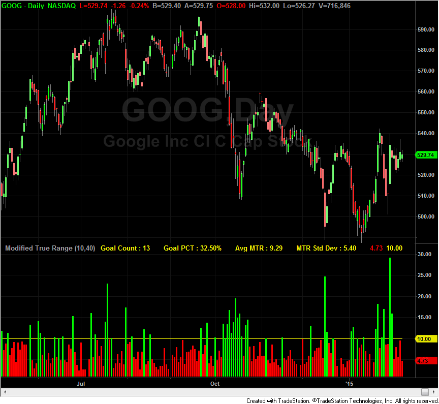
A sample chart is shown in Figure 1.

FIGURE 1: TRADESTATION, MODIFIED TRUE RANGE. Here is an example of the modified true range indicator applied to a daily chart of Google (GOOG).

This article is for informational purposes. No type of trading or investment recommendation, advice, or strategy is being made, given, or in any manner provided by TradeStation Securities or its affiliates.

—Doug McCrary
TradeStation Securities, Inc.
www.TradeStation.com

BACK TO LIST

eSIGNAL: APRIL 2015

For this month’s Traders’ Tip we’ve provided the formula ModifiedTrueRange.efs based on the formula described in Chris Lindgren’s article in the February 2015 issue of S&C, “Kiss & Touch With The Modified True Range.”

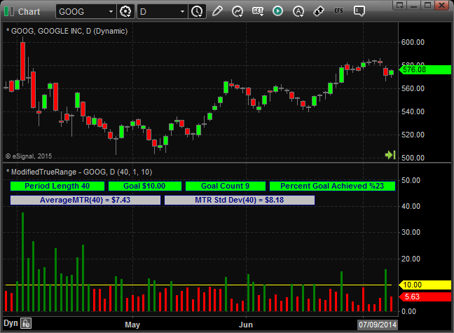
The study contains formula parameters to set the desired period and price, which may be configured through the edit chart window (right-click on the chart and select edit chart) to set the desired period and price. A sample chart is shown in Figure 2.

FIGURE 2: eSIGNAL, MODIFIED TRUE RANGE. Here is an example of the study on a chart of Google.

To discuss this study or download a complete copy of the formula code, please visit the EFS library discussion board forum under the forums link from the support menu at www.esignal.com or visit our EFS KnowledgeBase at https://www.esignal.com/support/kb/efs/. The eSignal formula script (EFS) is also available for copying & pasting here:

/*********************************
Provided By:  
    Interactive Data Corporation (Copyright © 2015) 
    All rights reserved. This sample eSignal Formula Script (EFS)
    is for educational purposes only. Interactive Data Corporation
    reserves the right to modify and overwrite this EFS file with 
    each new release. 

Description:        
    Kiss & Touch With The Modified True Range by Chris Lindgren
    
Version:            1.00  02/06/2015

Formula Parameters:                     Default:
Period                                  20 
Grouping Offset                         1
Goal                                    9.99

Notes:
    The related article is copyrighted material. If you are not a subscriber
    of Stocks & Commodities, please visit www.traders.com.

**********************************/

var fpArray = new Array();


function preMain(){

    
    setStudyTitle("ModifiedTrueRange");

    
    setCursorLabelName("GoalLevel", 0);
    setCursorLabelName("MTR", 1);
    
    setDefaultBarFgColor(Color.yellow, 0);
    setDefaultBarFgColor(Color.grey, 1);

    setPlotType(PLOTTYPE_LINE, 0);
    setPlotType(PLOTTYPE_HISTOGRAM, 1);

    setDefaultBarThickness(1, 0);
    setDefaultBarThickness(3, 1);

    var x = 0;

    fpArray[x] = new FunctionParameter("fpPeriod", FunctionParameter.NUMBER);
    with(fpArray[x++]){
        setName("Period");
        setLowerLimit(1);
        setDefault(20);
    }

    fpArray[x] = new FunctionParameter("fpGroupOffset", FunctionParameter.NUMBER);
    with(fpArray[x++]){
        setName("Grouping Offset");
        setLowerLimit(1); 
        setDefault(1);
    }

    fpArray[x] = new FunctionParameter("fpGoal", FunctionParameter.NUMBER);
    with(fpArray[x++]){
        setName("Goal");
        setLowerLimit(0);
        setDefault(9.99);
    } 
}

var bInit = false;
var bVersion = null;

var xClose = null;
var xLowest = null;
var xHighest = null;

var xRanges = null;



var xMTR = null;

var xRange = null;



var xHitGoal = null;

var xAvgMTR = null;
var xMTRStdDev = null;



var aLabels = [];

var nButtonSpace = 5;


function main(fpPeriod, fpGroupOffset, fpGoal){

    
    if (bVersion == null) bVersion = verify();
    if (bVersion == false) return;

    if (!bInit){
    	xClose = close();
    	xLowest = lowest(fpGroupOffset, low());

        xHighest = highest(fpGroupOffset, high());

        xRanges = efsInternal("Calc_Ranges", xClose, xLowest, xHighest, fpGroupOffset);

        

        xMTR = getSeries(xRanges, 0);

        xRange = getSeries(xRanges, 1);

        

        xHitGoal = efsInternal("Calc_HitGoal", xMTR, fpGoal);

        

        xAvgMTR = sma(fpPeriod, xMTR);

        xMTRStdDev = efsInternal("Calc_StdDev", xRange, fpPeriod);

        
        bInit = true; 
    }
  
    var nMTR = xMTR.getValue(0);

    if (nMTR == null)

        return;

    setBarFgColor((nMTR >= fpGoal) ? Color.green : Color.red, 1);

        

    var GoalCount = null;

    for (var i = 0; i < fpPeriod; i++){

        var nHitGoal = xHitGoal.getValue(-i);

        if (nHitGoal == null){

            GoalCount = "n/a"

            break;

        }

        GoalCount += nHitGoal;

    }

        

    var GoalPct = (GoalCount == "n/a") ? "n/a" : "%" + Math.round(GoalCount / fpPeriod * 100);



    var AvgMTR = xAvgMTR.getValue(0);

    var MTRStdDev = xMTRStdDev.getValue(0);

    

    AvgMTR = (AvgMTR == null) ? "n/a" : "$" + AvgMTR.toFixed(2);

    MTRStdDev = (MTRStdDev == null) ? "n/a" : "$" + MTRStdDev.toFixed(2);

        

    if (isLastBarOnChart()){

        var x = 10;

        var y = 25;

            

        aLabels = [];

        aLabels.push((fpGroupOffset > 1) ? 

        ["** Special Grouping is set is for " + fpGroupOffset + " bars **", 285, Color.RGB(255,155,0)] : null);

        aLabels.push(["Period Length " + fpPeriod, 135, Color.lime]);

        aLabels.push(["Goal $" + fpGoal.toFixed(2), 105, Color.lime]);

        aLabels.push(["Goal Count " + GoalCount, 115, Color.lime]);

        aLabels.push(["Percent Goal Achieved " + GoalPct, 180, Color.lime]);

        aLabels.push(["AverageMTR(" + fpPeriod + ") = " + AvgMTR, 215, Color.lightgrey]);

        aLabels.push(["MTR Std Dev(" + fpPeriod + ") = " + MTRStdDev, 215, Color.lightgrey]);

    

        aLabels.forEach(

            function(aValue, nIndex){

                if (aValue != null){

                    drawTextPixel(x, y, aValue[0], Color.navy, aValue[2],

                    Text.BOLD|Text.FRAME|Text.CENTER, "Arial", 8, aValue[0], aValue[1]);

                    x = x + aValue[1] + nButtonSpace;

                }

                if (nIndex == 4){

                    x = 10;

                    y = 45;

                }

            } 

        )

    } 

    
    return [fpGoal, nMTR]; 
}


function Calc_Ranges(xClose, xLowest, xHighest, nGroupOffset){

    

    nPrevClose = xClose.getValue(-nGroupOffset);

    nLowest = xLowest.getValue(0);

    nHighest = xHighest.getValue(0);



    if (nPrevClose == null || nLowest == null || nHighest == null) 

        return;



    var nRangeLow = Math.abs(nPrevClose - nLowest);

    var nRangeHigh = Math.abs(nPrevClose - nHighest);

    

    var nMTR = Math.max(nRangeLow, nRangeHigh);

    

    var nRangeLow1 = (nPrevClose - nLowest);

    var nRangeHigh1 = (nPrevClose - nHighest);

    

    var nRange = Math.abs(nRangeLow1) >= Math.abs(nRangeHigh1) ? nRangeLow1 : nRangeHigh1;

    

    return [nMTR, nRange];

}



function Calc_StdDev(xSource, nPeriod){

    

    var nSumX = 0; 

    var nSumX2 = 0; 



    for (i = 0; i < nPeriod; i++){ 

        var nSource = xSource.getValue(-i);

        if (nSource == null)

            return;

        nSumX += nSource; 

        nSumX2 += (nSource * nSource); 

    } 



    var nSMA = (nSumX / nPeriod); 

    var nStdDev = Math.sqrt((nSumX2 / nPeriod) - (nSMA * nSMA)); 



    return nStdDev; 

}


function Calc_HitGoal(xMTR, nGoal){

    

    var nMTR = xMTR.getValue(0);

        

    if (nMTR == null)

        return;

    

    var nHitGoal = (nMTR >= nGoal) ? 1 : 0;

   

    return nHitGoal;

}


function verify(){

    
    var b = false;
    if (getBuildNumber() < 779){
        drawTextAbsolute(5, 35, "This study requires version 8.0 or later.", 
            Color.white, Color.blue, Text.RELATIVETOBOTTOM|Text.RELATIVETOLEFT|Text.BOLD|Text.LEFT,
            null, 13, "error");
        drawTextAbsolute(5, 20, "Click HERE to upgrade.@URL=https://www.esignal.com/download/default.asp", 
            Color.white, Color.blue, Text.RELATIVETOBOTTOM|Text.RELATIVETOLEFT|Text.BOLD|Text.LEFT,
            null, 13, "upgrade");
        return b;
    } 
    else 
        b = true;

    return b;
}

—Eric Lippert
eSignal, an Interactive Data company
800 779-6555, www.eSignal.com

BACK TO LIST

WEALTH-LAB: APRIL 2015

In his February 2015 S&C article, “Kiss & Touch With The Modified True Range,” author Chris Lindgren explored an option’s probability of reaching a certain price prior to expiration. Figuring the probability is achieved through some simple statistical calculations. At the foundation of his work is a new rendition of J. Welles Wilder’s classic indicator true range (TR) referred to in Lingren’s articles as the modified true range (MTR). The difference between the true range and the modified true range is simply the omission of the current high less the current low. Lindgren’s new indicator only considers the greatest of the following two values:

Absolute value of the current high less the previous close
Absolute value of the current low less the previous close

It’s noticeable how the rounding performed by the average MTR indicator makes the result appear smoother than the traditional average true range (ATR).

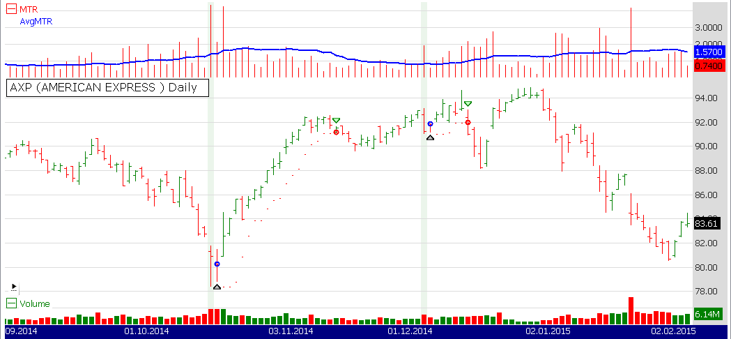
While option trading is an interesting topic of its own, here we will explore applications of the indicator introduced by Lindgren to trading securities. One example of a possible trading idea could be detection of price spikes using the new MTR indicator. Our sample trading system will follow a countertrend, mean-reversion approach, fading strong moves over a short-term horizon. To spot outlier values in the price, we calculate the standard deviation of the MTR. The setup is in place when the current MTR reading exceeds the average MTR by three standard deviations of MTR or greater. An entry is triggered when the following criteria are met:

Buy next bar at market if today’s close price has declined
Short next bar at market if today’s close price has increased.

A position is exited with a simple trailing channel exit:

Exit long when today’s low price has broken below the three-day lowest price
Cover short when today’s high price has broken above the three-day highest price.

See Figure 3 for an example chart.

FIGURE 3: WEALTH-LAB, MODIFIED TRUE RANGE. This sample Wealth-Lab 6 chart illustrates the sample system’s performance on a daily chart of American Express (AXP).

This system is merely a proof-of-concept. Among possible enhancements to this barebone system, consider the following suggestions:

Perform trend detection to avoid entering against established trends
To support the trailing exit, introduce a stop-loss for risk management
Explore whether “clumping” of MTR spikes has an effect on the system’s profitability.

Wealth-Lab 6 strategy code (C#):

using System;
using System.Collections.Generic;
using System.Text;
using System.Drawing;
using WealthLab;
using WealthLab.Indicators;

namespace WealthLab.Strategies
{
	public class ModifiedTrueRange : WealthScript
	{
		private StrategyParameter paramPeriod;

		public ModifiedTrueRange()
		{
			paramPeriod = CreateParameter("Period", 20, 1, 100, 1);
		}

		protected override void Execute()
		{
			int period = paramPeriod.ValueInt;
			double Goal = 9.99;

			//Calcluate modified true range (MTR)

			DataSeries MTR = new DataSeries( Bars,"MTR" );
			DataSeries RangeLow = DataSeries.Abs( (Close>>1)-Lowest.Series(Low,1) );
			DataSeries RangeHigh = DataSeries.Abs( (Close>>1)-Highest.Series(High,1) );
			DataSeries Range1 = new DataSeries( Bars,"Range" );
			DataSeries HitGoal = new DataSeries( Bars,"HitGoal" );
			DataSeries GoalCount = new DataSeries( Bars,"GoalCount" );
			DataSeries GoalPct = new DataSeries( Bars,"GoalPct" );
			DataSeries AvgMTR = new DataSeries( Bars,"AvgMTR" );
			
			for(int bar = 1; bar < Bars.Count; bar++)
			{
				double mtr = Math.Max(RangeLow[bar],RangeHigh[bar]);
				MTR[bar] = mtr;
			}

			//MTR Standard Deviation

			DataSeries RangeLow1=( (Close>>1) - Lowest.Series(Low,1) );
			DataSeries RangeHigh1=( (Close>>1) - Highest.Series(High,1) );

			for(int bar = 1; bar < Bars.Count; bar++)
			{
				double range = ( Math.Abs(RangeLow1[bar]) >= Math.Abs(RangeHigh1[bar]) ) ?
					RangeLow1[bar] : RangeHigh1[bar];					
				Range1[bar] = range;
			}

			DataSeries MTRStdDev = StdDev.Series(Range1,period,StdDevCalculation.Sample);

			for(int bar = 1; bar < Bars.Count; bar++)
			{
				HitGoal[bar] = MTR[bar] >= Goal ? 1 : 0;
				GoalCount[bar] = Sum.Series( HitGoal,period )[bar];
				
				double goalPct = Math.Round( GoalCount[bar]/period, 2) * 100;
				double avgMTR = Math.Round( SMA.Series(MTR,period)[bar], 2 );
				
				GoalPct[bar] = goalPct;
				AvgMTR[bar] = avgMTR;
			}
			
			StdDev MTRSD = StdDev.Series(MTR,period,StdDevCalculation.Sample);
			
			ChartPane mtrPane = CreatePane( 40, true, true );
			PlotSeries( mtrPane, MTR, Color.Red, LineStyle.Histogram, 1 );
			PlotSeries( mtrPane, AvgMTR, Color.Blue, LineStyle.Solid, 2 );
			PlotStops();

			for(int bar = GetTradingLoopStartBar(period); bar < Bars.Count; bar++)
			{
				if (IsLastPositionActive)
				{
					Position p = LastPosition;
					if( p.PositionType == PositionType.Long )
						SellAtStop( bar+1, p, Lowest.Series( Low,3 )[bar] );
					else
						CoverAtStop( bar+1, p, Highest.Series( High,3 )[bar] );
				}
				else
				{
					//MTR spike
					bool spike = MTR[bar] > (AvgMTR[bar] + 3 * MTRSD[bar]);
					if( spike )
					{
						SetBackgroundColor( bar, Color.FromArgb( 20, Color.Green ) );
						if( ROC.Value( bar, Close, 1 ) > 0 )
							ShortAtMarket(bar+1 );
						else
							BuyAtMarket(bar+1 );
					}
				}
			}
		}
	}
}

—Eugene, Wealth-Lab team
MS123, LLC
www.wealth-lab.com

BACK TO LIST

NEUROSHELL TRADER: APRIL 2015

An RSI mean-reverting basket trading system such as the one described in Dave Cline’s article in this issue, “Basket Trading Using A Directed Acyclic Graph,” can be easily implemented with a few of NeuroShell Trader’s 800+ indicators. Simply select new trading strategy from the insert menu and enter the following in the appropriate locations of NeuroShell’s trading strategy wizard:

BUY LONG CONDITIONS:            A<=B(ChartPageURank(RSI(Close,5)),3)
SELL LONG CONDITIONS:      	A>B(ChartPageURank(RSI(Close,5)),3)
SELL SHORT CONDITIONS:    	A<=B(ChartPageLRank(RSI(Close,5)),3)
COVER SHORT CONDITIONS: 	A>B(ChartPageLRank(RSI(Close,5)),3)

If you have NeuroShell Trader Professional, you can also choose whether the parameters should be optimized. After backtesting the trading strategy, use the detailed analysis button to view the backtest and trade-by-trade statistics for the strategy.

Users of NeuroShell Trader can go to the Stocks & Commodities section of the NeuroShell Trader free technical support website to download a copy of this or any previous Traders’ Tips.

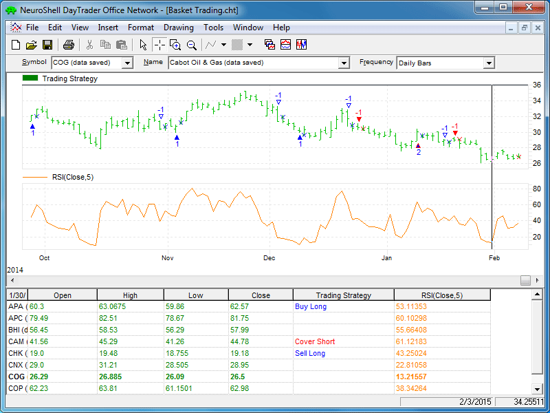
A sample chart is shown in Figure 4.

FIGURE 4: NEUROSHELL TRADER, BASKET TRADING SYSTEM. This NeuroShell Trader chart displays an RSI mean-reverting basket trading system.

—Marge Sherald, Ward Systems Group, Inc.
301 662-7950, sales@wardsystems.com
www.neuroshell.com

BACK TO LIST

AIQ: APRIL 2015

The AIQ code based on Dave Cline’s article in this issue, “Basket Trading Using A Directed Acyclic Graph,” is provided at www.TradersEdgeSystems.com/traderstips.htm, and is also shown here:


!BASKET TRADING USING A DIRECTED ACYCLIC GRAPH

!Author: Dave Cline, TASC April 2015

!Coded by: Richard Denning 2/10/2015

!www.TradersEdgeSystems.com



!Len is the number of lookback days.

!L1 is the first ticker in the list that you want to compare your list to.

!L2 is the second ticker in the list that you want to compare your list to etc

!You must create a list of 20 or less symbols of interest then type in the same 

!symbols in the same alpha order as your list. If there are less than 20 just use " "

!but do not delete the input as there must be L1 through L20 inputs defined:



!INPUTS: 

Len is 250.

L1 is "ADBE".

L2 is "ADI".

L3 is "ADP".

L4 is "AKAM".

L5 is "ALTR".

L6 is "AMAT".

L7 is "FOX".

L8 is "INTU".

L9 is "LLTC".

L10 is "LMCA".

L11 is "LRCX".

L12 is "LVNTA".

L13 is "NTAP".

L14 is "NVDA".

L15 is "NXPI".

L16 is "PAYX".

L17 is "SIRI".

L18 is "TRIP".

L19 is "TXN".

L20 is "VIAB".



!CODE TO CALCULATE PEARSONS r AND r SQUARED:

ChgOC is (([close]-[open])/[open]) * 100.

SumY is Sum(ChgOC, Len).

SumYsq is Sum(ChgOC*ChgOC, Len).

SSy is SumYsq - ( (SumY * SumY) / Len ).



ChgOCL1 is TickerUDF(L1, ChgOC).

SumXsq1 is Sum(ChgOCL1*ChgOCL1, Len).

SumX1 is Sum(ChgOCL1, Len).

SumXY1 is Sum(ChgOC*ChgOCL1, Len).

SP1 is SumXY1 - ( (SumX1 * SumY) / Len ).

SSx1 is SumXsq1 - ( (SumX1 * SumX1) / Len ).

PearR1 is SP1/SQRT(SSx1*SSy).

PearRsq1 is ( PearR1 * PearR1 ).



ChgOCL2 is TickerUDF(L2, ChgOC).

SumXsq2 is Sum(ChgOCL2*ChgOCL2, Len).

SumX2 is Sum(ChgOCL2, Len).

SumXY2 is Sum(ChgOC*ChgOCL2, Len).

SP2 is SumXY2 - ( (SumX2 * SumY) / Len ).

SSx2 is SumXsq2 - ( (SumX2 * SumX2) / Len ).

PearR2 is SP2/SQRT(SSx2*SSy).

PearRsq2 is ( PearR2 * PearR2 ).



ChgOCL3 is TickerUDF(L3, ChgOC).

SumXsq3 is Sum(ChgOCL3*ChgOCL3, Len).

SumX3 is Sum(ChgOCL3, Len).

SumXY3 is Sum(ChgOC*ChgOCL3, Len).

SP3 is SumXY3 - ( (SumX3 * SumY) / Len ).

SSx3 is SumXsq3 - ( (SumX3 * SumX3) / Len ).

PearR3 is SP3/SQRT(SSx3*SSy).

PearRsq3 is ( PearR3 * PearR3 ).



ChgOCL4 is TickerUDF(L4, ChgOC).

SumXsq4 is Sum(ChgOCL4*ChgOCL4, Len).

SumX4 is Sum(ChgOCL4, Len).

SumXY4 is Sum(ChgOC*ChgOCL4, Len).

SP4 is SumXY4 - ( (SumX4 * SumY) / Len ).

SSx4 is SumXsq4 - ( (SumX4 * SumX4) / Len ).

PearR4 is SP4/SQRT(SSx4*SSy).

PearRsq4 is ( PearR4 * PearR4 ).



ChgOCL5 is TickerUDF(L5, ChgOC).

SumXsq5 is Sum(ChgOCL5*ChgOCL5, Len).

SumX5 is Sum(ChgOCL5, Len).

SumXY5 is Sum(ChgOC*ChgOCL5, Len).

SP5 is SumXY5 - ( (SumX5 * SumY) / Len ).

SSx5 is SumXsq5 - ( (SumX5 * SumX5) / Len ).

PearR5 is SP5/SQRT(SSx5*SSy).

PearRsq5 is ( PearR5 * PearR5 ).



ChgOCL6 is TickerUDF(L6, ChgOC).

SumXsq6 is Sum(ChgOCL6*ChgOCL6, Len).

SumX6 is Sum(ChgOCL6, Len).

SumXY6 is Sum(ChgOC*ChgOCL6, Len).

SP6 is SumXY6 - ( (SumX6 * SumY) / Len ).

SSx6 is SumXsq6 - ( (SumX6 * SumX6) / Len ).

PearR6 is SP6/SQRT(SSx6*SSy).

PearRsq6 is ( PearR6 * PearR6 ).



ChgOCL7 is TickerUDF(L7, ChgOC).

SumXsq7 is Sum(ChgOCL7*ChgOCL7, Len).

SumX7 is Sum(ChgOCL7, Len).

SumXY7 is Sum(ChgOC*ChgOCL7, Len).

SP7 is SumXY7 - ( (SumX7 * SumY) / Len ).

SSx7 is SumXsq7 - ( (SumX7 * SumX7) / Len ).

PearR7 is SP7/SQRT(SSx7*SSy).

PearRsq7 is ( PearR7 * PearR7 ).



ChgOCL8 is TickerUDF(L8, ChgOC).

SumXsq8 is Sum(ChgOCL8*ChgOCL8, Len).

SumX8 is Sum(ChgOCL8, Len).

SumXY8 is Sum(ChgOC*ChgOCL8, Len).

SP8 is SumXY8 - ( (SumX8 * SumY) / Len ).

SSx8 is SumXsq8 - ( (SumX8 * SumX8) / Len ).

PearR8 is SP8/SQRT(SSx8*SSy).

PearRsq8 is ( PearR8 * PearR8 ).



ChgOCL9 is TickerUDF(L9, ChgOC).

SumXsq9 is Sum(ChgOCL9*ChgOCL9, Len).

SumX9 is Sum(ChgOCL9, Len).

SumXY9 is Sum(ChgOC*ChgOCL9, Len).

SP9 is SumXY9 - ( (SumX9 * SumY) / Len ).

SSx9 is SumXsq9 - ( (SumX9 * SumX9) / Len ).

PearR9 is SP9/SQRT(SSx9*SSy).

PearRsq9 is ( PearR9 * PearR9 ).



ChgOCL10 is TickerUDF(L10, ChgOC).

SumXsq10 is Sum(ChgOCL10*ChgOCL10, Len).

SumX10 is Sum(ChgOCL10, Len).

SumXY10 is Sum(ChgOC*ChgOCL10, Len).

SP10 is SumXY10 - ( (SumX10 * SumY) / Len ).

SSx10 is SumXsq10 - ( (SumX10 * SumX10) / Len ).

PearR10 is SP10/SQRT(SSx10*SSy).

PearRsq10 is ( PearR10 * PearR10 ).



ChgOCL11 is TickerUDF(L11, ChgOC).

SumXsq11 is Sum(ChgOCL11*ChgOCL11, Len).

SumX11 is Sum(ChgOCL11, Len).

SumXY11 is Sum(ChgOC*ChgOCL11, Len).

SP11 is SumXY11 - ( (SumX11 * SumY) / Len ).

SSx11 is SumXsq11 - ( (SumX11 * SumX11) / Len ).

PearR11 is SP11/SQRT(SSx11*SSy).

PearRsq11 is ( PearR11 * PearR11 ).



ChgOCL12 is TickerUDF(L12, ChgOC).

SumXsq12 is Sum(ChgOCL12*ChgOCL12, Len).

SumX12 is Sum(ChgOCL12, Len).

SumXY12 is Sum(ChgOC*ChgOCL12, Len).

SP12 is SumXY12 - ( (SumX12 * SumY) / Len ).

SSx12 is SumXsq12 - ( (SumX12 * SumX12) / Len ).

PearR12 is SP12/SQRT(SSx12*SSy).

PearRsq12 is ( PearR12 * PearR12 ).



ChgOCL13 is TickerUDF(L13, ChgOC).

SumXsq13 is Sum(ChgOCL13*ChgOCL13, Len).

SumX13 is Sum(ChgOCL13, Len).

SumXY13 is Sum(ChgOC*ChgOCL13, Len).

SP13 is SumXY13 - ( (SumX13 * SumY) / Len ).

SSx13 is SumXsq13 - ( (SumX13 * SumX13) / Len ).

PearR13 is SP13/SQRT(SSx13*SSy).

PearRsq13 is ( PearR13 * PearR13 ).



ChgOCL14 is TickerUDF(L14, ChgOC).

SumXsq14 is Sum(ChgOCL14*ChgOCL14, Len).

SumX14 is Sum(ChgOCL14, Len).

SumXY14 is Sum(ChgOC*ChgOCL14, Len).

SP14 is SumXY14 - ( (SumX14 * SumY) / Len ).

SSx14 is SumXsq14 - ( (SumX14 * SumX14) / Len ).

PearR14 is SP14/SQRT(SSx14*SSy).

PearRsq14 is ( PearR14 * PearR14 ).



ChgOCL15 is TickerUDF(L15, ChgOC).

SumXsq15 is Sum(ChgOCL15*ChgOCL15, Len).

SumX15 is Sum(ChgOCL15, Len).

SumXY15 is Sum(ChgOC*ChgOCL15, Len).

SP15 is SumXY15 - ( (SumX15 * SumY) / Len ).

SSx15 is SumXsq15 - ( (SumX15 * SumX15) / Len ).

PearR15 is SP15/SQRT(SSx15*SSy).

PearRsq15 is ( PearR15 * PearR15 ).



ChgOCL16 is TickerUDF(L16, ChgOC).

SumXsq16 is Sum(ChgOCL16*ChgOCL16, Len).

SumX16 is Sum(ChgOCL16, Len).

SumXY16 is Sum(ChgOC*ChgOCL16, Len).

SP16 is SumXY16 - ( (SumX16 * SumY) / Len ).

SSx16 is SumXsq16 - ( (SumX16 * SumX16) / Len ).

PearR16 is SP16/SQRT(SSx16*SSy).

PearRsq16 is ( PearR16 * PearR16 ).



ChgOCL17 is TickerUDF(L17, ChgOC).

SumXsq17 is Sum(ChgOCL17*ChgOCL17, Len).

SumX17 is Sum(ChgOCL17, Len).

SumXY17 is Sum(ChgOC*ChgOCL17, Len).

SP17 is SumXY17 - ( (SumX17 * SumY) / Len ).

SSx17 is SumXsq17 - ( (SumX17 * SumX17) / Len ).

PearR17 is SP17/SQRT(SSx17*SSy).

PearRsq17 is ( PearR17 * PearR17 ).



ChgOCL18 is TickerUDF(L18, ChgOC).

SumXsq18 is Sum(ChgOCL18*ChgOCL18, Len).

SumX18 is Sum(ChgOCL18, Len).

SumXY18 is Sum(ChgOC*ChgOCL18, Len).

SP18 is SumXY18 - ( (SumX18 * SumY) / Len ).

SSx18 is SumXsq18 - ( (SumX18 * SumX18) / Len ).

PearR18 is SP18/SQRT(SSx18*SSy).

PearRsq18 is ( PearR18 * PearR18 ).



ChgOCL19 is TickerUDF(L19, ChgOC).

SumXsq19 is Sum(ChgOCL19*ChgOCL19, Len).

SumX19 is Sum(ChgOCL19, Len).

SumXY19 is Sum(ChgOC*ChgOCL19, Len).

SP19 is SumXY19 - ( (SumX19 * SumY) / Len ).

SSx19 is SumXsq19 - ( (SumX19 * SumX19) / Len ).

PearR19 is SP19/SQRT(SSx19*SSy).

PearRsq19 is ( PearR19 * PearR19 ).



ChgOCL20 is TickerUDF(L20, ChgOC).

SumXsq20 is Sum(ChgOCL20*ChgOCL20, Len).

SumX20 is Sum(ChgOCL20, Len).

SumXY20 is Sum(ChgOC*ChgOCL20, Len).

SP20 is SumXY20 - ( (SumX20 * SumY) / Len ).

SSx20 is SumXsq20 - ( (SumX20 * SumX20) / Len ).

PearR20 is SP20/SQRT(SSx20*SSy).

PearRsq20 is ( PearR20 * PearR20 ).



!REPORTS TO DISPLAY VALUES"

PearsonR if 1=1.

PearsonRsq if 1=1.

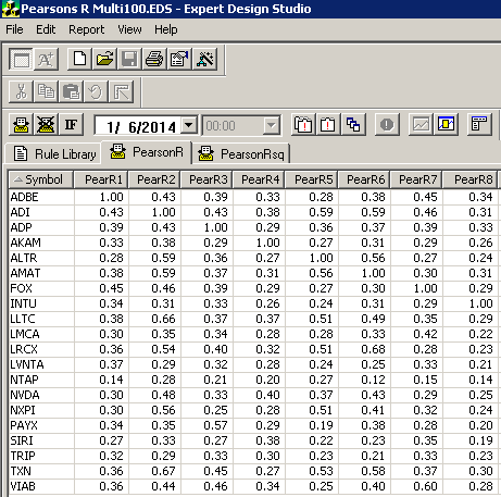
The code provided will compute the Pearson correlation or “r” between two pairs of stocks for up to 20 stocks at a time. The EDS reports can be exported to Excel for further analysis. I used the AIQ Matchmaker module, which uses Spearman rank correlation to find highly correlated stocks from within the NASDAQ 100. I then created a list of these 20 symbols and set the EDS file to run only on this list. I then typed in the list in the same alphabetic order as they are in the list. I then set the report date to 1/6/2014, which is about one year prior to when I was writing this. The correlations are set to look back 250 days based on the input “len.” Once we have decided how we will trade the basket created by the correlation analysis, we would forward-test using data not used to correlate the stocks, or from 1/7/2014 to 1/8/2015.

FIGURE 5: AIQ, CORRELATION REPORT. This shows a portion of the correlation matrix report that is created from the AIQ EDS code for 20 of the NASDAQ 100 stocks in my sample test.

Figure 5 shows a portion of the resulting report. The cells with a 1.00 value are the result of correlating the stock with itself. Since the column headings use a variable name, the cells with the 1.00 value identify the stock in that column. This matrix can be used to create the correlated baskets described by the author. I also created a report for Pearson’s r squared, but this is not used by Cline in his article.

—Richard Denning
info@TradersEdgeSystems.com
for AIQ Systems

BACK TO LIST

TRADERSSTUDIO: APRIL 2015

The TradersStudio code for Dave Cline’s article in this issue, “Basket Trading Using A Directed Acyclic Graph,” can be found at:

The following code file is provided in the download:

System: BASKET—A long-only system that uses daily data and buys all stocks that are set up in the session data list. There are no exits, as this is used solely for getting the complete set of correlation values for each pair.

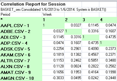
The purpose of the very simple code I am providing is to get the “Eq Correlation” report to run on the entire period based on the start/end dates input in the session backtest for the entire list of stocks in the session. Note that the correlation report is based on a proprietary correlation formula that is similar to Pearson’s r.

The TradersStudio code is as follows:


'BASKET TRADING USING A DIRECTED ACYCLIC GRAPH

'Author: Dave Cline, TASC April 2015

'Coded by: Richard Denning 2/10/2015

'www.TradersEdgeSystems.com



sub BASKET()

If 1=1 Then Buy("LE",1,0,Market,Day)

End Sub

Figure 6 shows a portion of the EQ Correlation report that I ran on the NASDAQ 100 stocks for the period from 1/6/2013 to 1/6/2014. The cells with a “1” value are the result of correlating the stock with itself. Since the column headings use a variable name, the cells with the “1” value identify the stock in that column. This matrix can be used to create the correlated baskets described by the author. The report can be saved to an Excel file for further analysis of the pairs.

FIGURE 6: TRADERSSTUDIO, CORRELATION REPORT. This shows a portion of the EQ Correlation report that I ran on the NASDAQ 100 stocks for the period from 1/6/2013 to 1/6/2014.

—Richard Denning
info@TradersEdgeSystems.com
for TradersStudio

BACK TO LIST

UPDATA: APRIL 2015

Our Traders’ Tip for this month is a system found in the Updata library, named breadth correlation system.

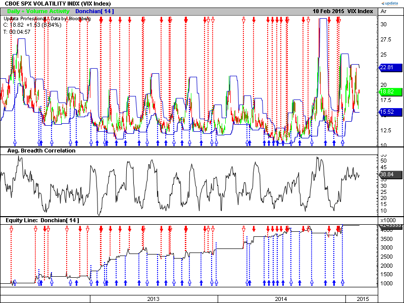
This system measures the average correlation of S&P 500 Index constituents to the VIX Index future. If this correlation falls below a certain level, then Donchian channels are used to give signals for market entry, assuming that the cyclical correlation value will eventually rise, and that periods of high correlation are also trending phases for the market. Exits are on a fixed number of days, proportional in number to the Donchian period.

FIGURE 7: UPDATA, BREADTH CORRELATION. This chart shows the breadth correlation system as applied to the rolling VIX future, of daily resolution.

The Updata code for this article can be found in the Updata library and may be downloaded by clicking the custom menu and system library. Those who cannot access the library due to a firewall may paste the code shown here into the Updata custom editor and save it.

PARAMETER "WatchList" &MyList=SELECT  
PARAMETER "Period" #PERIOD=14 
PARAMETER "RsQ Thresh." @THRESH=30 
DISPLAYSTYLE 3LINES
INDICATORTYPE TOOL
INDICATORTYPE3 CHART  
COLOUR RGB(0,0,200) 
COLOUR2 RGB(0,0,200)
NAME "Donchian[" #PERIOD "]" ""
NAME3 "Avg. Breadth Correlation" ""
#TICKERNUMBER=0 
#COUNT=0  
@CORRELSUM=0
@PeriodUpper=0
@PeriodLower=0
FOR #CURDATE=#PERIOD TO #LASTDATE
   'VARIABLES
   #COUNT=0
   @CORRELSUM=0 
   @PeriodUpper=PHIGH(HIGH(1),#PERIOD,1)
   @PeriodLower=PLOW(LOW(1),#PERIOD,1)
   'AVG THE CORRELATION STATISTIC ACROSS THE WATCHLIST
   FOR #TICKERNUMBER=0 to LENGTH(&MyList)-1
       @CORRELSUM=@CORRELSUM+COEFFDET(CLOSE,CLOSE(&MyList,#TICKERNUMBER),#PERIOD)/(LENGTH(&MyList)-1)
   NEXT  
   'EXIT AFTER #PERIOD/2 BARS HELD
   IF ORDEROPENFOR>INT(#PERIOD/2) 
      COVER CLOSE  
      SELL CLOSE
   ENDIF  
   'SHORT ENTRY
   IF @CORRELSUM<@THRESH AND CLOSE<@PeriodLower
      BUY CLOSE 
   ENDIF 
   'LONG ENTRY
   IF @CORRELSUM<@THRESH AND CLOSE>@PeriodUpper
      SHORT CLOSE 
   ENDIF       
   'PLOT LINES
   @PLOT3=@CORRELSUM  
   @PLOT=@PeriodUpper
   @PLOT2=@PeriodLower    
NEXT

—Updata support team
support@updata.co.uk, www.updata.co.uk

BACK TO LIST

MICROSOFT EXCEL: APRIL 2015

The article “Basket Trading Using A Directed Acyclic Graph” by Dave Cline in this issue is the proverbial duck on a pond: At first glance, it’s an interesting introduction to basket trading. But under the surface, a closer reading shows there is a lot of work that must go into preparing our trading basket before we can start trading.

Cline’s article describes three rather sizeable pieces:

1. Build a raw, pairwise correlation database from a user-supplied list of symbols.

Set a time window for sampling symbol correlations. This should be built on recent history for a live trading system. However, for backtesting, use period chosen should predate the intended backtest period.
Set the number of bars to be used for correlation calculations.
Set a correlation value threshold to filter out the worst-performing correlation pairs.
Perhaps further limit the list to the N pairs with the highest correlation values.

2. Use directed acyclic graph (DAG) processing to trim the correlations list built above into a sizeable list of symbols with strong mutual intercorrelations.

Notice that step 1 may give us “islands” of symbols with strong intercorrelations within the island. I call them islands because symbols in these groupings, while strongly intercorrelated among members of the containing island, will have no strong intercorrelations with symbols in any of the other islands. This is because any interconnections that may have existed between the separate groupings did not survive the correlation threshold filtering in step 1. In short, the islands do not correlate well with each other. They move in different ways.

Any one of these islands could be the basis of a basket trading group.

DAG critical path processing is intended to choose the largest possible set of the most strongly intercorrelated symbols; presumably, this set will come out of the island group with the strongest internal correlations.

Cline takes this one step further using the custom method GetLimitedNetworkedList as the last step of the DAG process to apply some additional filtering refinements.

3. Feed the resulting list of symbols to a basket trading system of your choice.

Any one of these three pieces represents a significant spreadsheet on its own. And none of them lends itself to being done purely, or even mostly, as spreadsheet cell formulas. Thus, the spreadsheet for this Traders’ Tip uses lots of VBA macro code.

The spreadsheet presented here tackles the first piece: building the correlation pairs database from a user-specified list of symbols.

My Figures 8–11 show steps of the process. My example uses a list of the symbols that constitute the S&P 500 index.

1. On the Internet, look up the constituent symbols list for the S&P 500.

Copy to a work area for manual cleanup efforts. In this case, a worksheet tab named “S&P 500 constituent symbols” serves as my work area.
Manually remove any embedded links that came with the copied list.
Manually remove extraneous stuff that also came with the copied list.
Adjust the symbol formats. A couple of the symbols contained periods, such as BRK.B and BF.B. Replace the periods with hyphens, which is the Yahoo Finance standard.

(See Figure 8.)

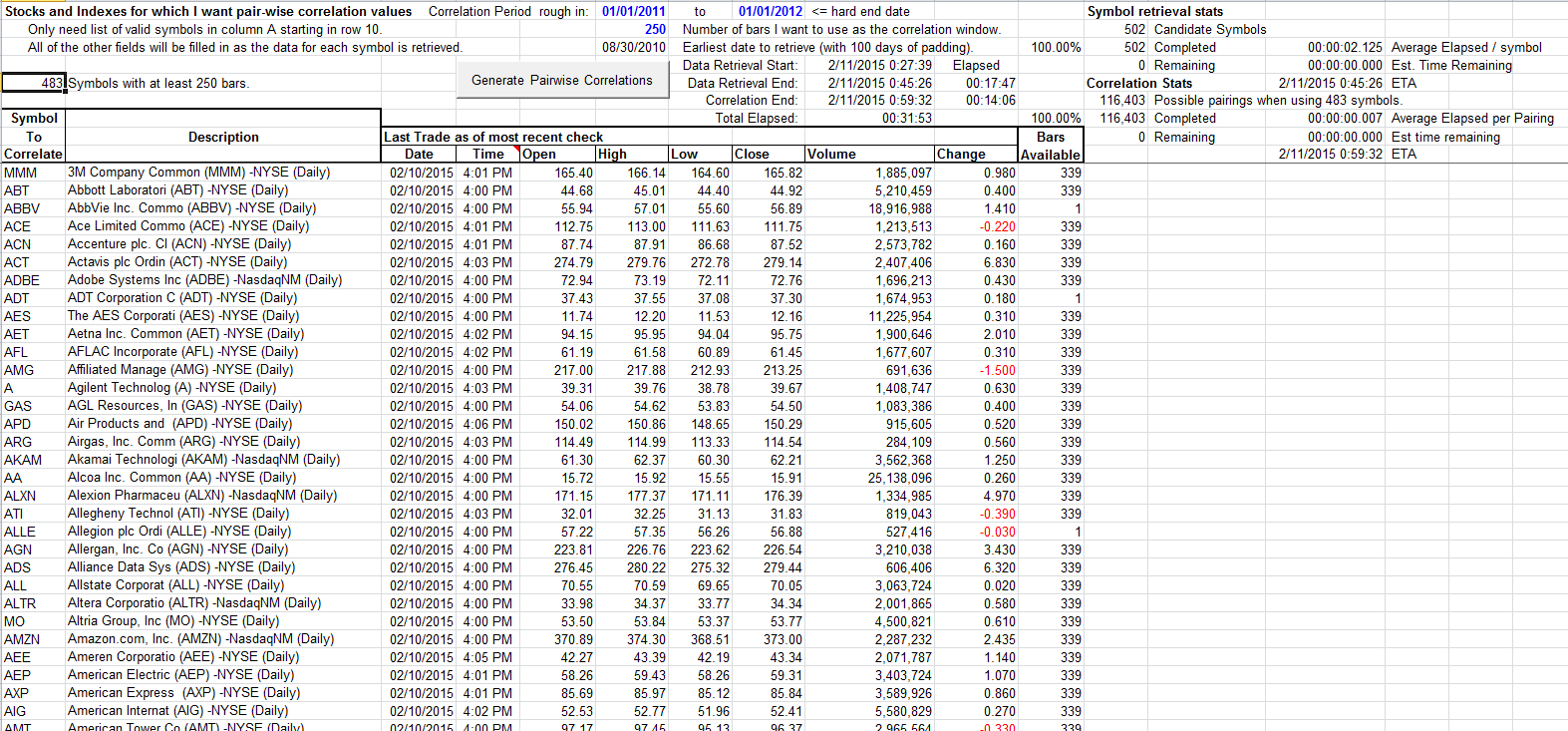
FIGURE 8: EXCEL, CORRELATION CANDIDATES. This shows the correlation candidates tab after a complete symbol retrieval and pair generation.

2. The CorrelationCandidates tab drives the process of downloading data for each of the candidate symbols. When the symbol download phase is complete, the generation of the raw correlation pairs list automatically begins on the RawCorrelations tab.

User steps:

On the CorrelationCandidates tab, manually ClearContents of all rows below the header row (that is, row 8 down).
Manually copy in the list of symbols you cleaned up in step 1 starting in cell A8.
Set the correlation bar count, which is the number of bars required from each symbol of a pair for the correlation calculation.
Set begin and end dates for the correlation period of interest. The end date is used directly along with the correlation bar count plus a 100-bar padding to calculate the earliest date to retrieve. Yahoo history retrievals will give us all available bars for the period marked out by the earliest and the end dates.
Click the “Generate pairwise correlations” button and go get lunch. This can take a while.

On my computer, late at night when it might be expected that the Yahoo servers and the Internet would perhaps be under less strain, the symbol retrieval phase (Figure 9) took almost 18 minutes for the 502 symbols in my list.

FIGURE 9: EXCEL, SYMBOL RETRIEVAL. Symbol retrieval is in flight. The status bar shows the phase progress and estimated time to completion.

The subsequent Correlation Pair Generation Phase (Figure 10) took an additional 14 minutes. Total elapsed time was about 31 minutes. Your mileage may vary.

FIGURE 10: EXCEL, CORRELATION PAIR GENERATION. Here is the correlation pair generation phase with progress and estimated time to completion in the status bar.

The macros that manage the two phases of this work place progress messages on the bottom status bar. This computation uses the average time for the items already processed in the current phase to project a time remaining and an ETA for completion of the phase.

3. For the last filtering step, go to the SortedFilteredCorrelation tab. This is very quick, so playing with what-if scenarios at this stage is not at all painful.

FIGURE11: EXCEL, READY FOR DAG PROCESSING. Here, the sorted and filtered correlation pairs are ready for DAG processing.

Set the two filter values to your taste (Figure 11).
1. Threshold is a value between 1 and -1.
2. A max entries value greater than zero says that if the threshold filter allows a sufficiently large result set, trim the result to the top MaxEntries pairs. A zero value says give me anything the threshold value passes.
Normal, highest correlation results are obtained by clicking on the get top correlations button. Here is what is happening in the spreadsheet:
1. Entries are sorted by correlation value in descending order.
2. Entries with a correlation value less than the threshold are removed from the bottom.
3. If Max Entries is not zero, then any entries more than Max Entries down the list are removed.
If you wish, the lowest correlation results may be obtained by clicking on the “Get Bottom Correlations” button.
1. Entries are sorted by correlation value in ascending order, weakest at the top.
2. Flip the sign on the threshold (-threshold).
3. Entries with a correlation value greater than the -threshold value are removed.
4. If Max Entries is not zero, then any entries more than Max Entries down the list are removed.

4. Finally, export this refined list to your DAG processor of choice to complete selection of a basket of symbols.

After a full S&P 500 run, the saved spreadsheet takes around 17 megabytes. To reduce this spreadsheet to a manageable download size, I have stripped out retrieved symbol data. The download should be something less than 800 kb stored on your drive.

For demonstration purposes, you can cut back on the number of symbols you place on the CorrelationCandidates tab. Ten to 20 symbols should make a reasonable demo run. And a sample run of that size will not eat as much wall time while it runs, or hard drive space when you store it.

The spreadsheet file for this Traders’ Tip can be downloaded here. To successfully download it, follow these steps:

Right-click on the Excel file link, then
Select “save as” (or “save target as”) to place a copy of the spreadsheet file on your hard drive.

—Ron McAllister
Excel and VBA programmer
rpmac_xltt@sprynet.com

BACK TO LIST