| METASTOCK | |
| MSX DLL C++ CODE | |
| HILBERT CHANNEL BREAKOUT INDICATOR | |
| HILBERT CHANNEL BREAKOUT SIGNAL | |
| BYTE INTO THE MARKET | |
| NEUROSHELL DAYTRADER PROFESSIONAL |
or return to December 2000 Contents
You can copy these formulas and programs for easy use in your spreadsheet or analysis software. Simply "select" the desired text by highlighting as you would in any word processing program, then use your standard key command for copy or choose "copy" from the browser menu. The copied text can then be "pasted" into any open spreadsheet or other software by selecting an insertion point and executing a paste command. By toggling back and forth between an application window and the open Web page, data can be transferred with ease.
This month's tips include formulas and programs for:
METASTOCK MSX DLL C++ CODE HILBERT CHANNEL BREAKOUT INDICATOR HILBERT CHANNEL BREAKOUT SIGNAL BYTE INTO THE MARKET NEUROSHELL DAYTRADER PROFESSIONAL or return to December 2000 Contents
GO BACKThe function, system, and indicator introduced in the article "Optimizing With Hilbert Indicators" by Roger Darley and the Traders' Tip "Refining The Hilbert Indicator" by John Ehlers, both of which appeared in the November 2000 STOCKS & COMMODITIES, can be created in MetaStock 7.0 or higher with the use of the new MetaStock External Function (MSX) DLL interface. The C++ code and MetaStock formula code is shown below.
METASTOCK
MSX DLL C++ CODE
// Main Calculation loop (begins after the fifth valid bar)
for( l_iCurrentBar = a_iFirstValid + 5; l_iCurrentBar <= a_iLastValid; l_iCurrentBar++ )
{
        // Set Previous Bar counter
l_iPreviousBar = l_iCurrentBar - 1;

        // Calculate Smoother and Detrender values
l_pdSmoother[l_iCurrentBar] = (4 * a_pfPrice[l_iCurrentBar] + 3 * a_pfPrice[l_iPreviousBar] + 2 *
    a_pfPrice[l_iCurrentBar - 2] + a_pfPrice[l_iCurrentBar - 3])/10;
l_pdDetrender[l_iCurrentBar] = (.25 * l_pdSmoother[l_iCurrentBar] + .75 * l_pdSmoother[l_iCurrentBar -
    2] - .75 * l_pdSmoother[l_iCurrentBar - 4] - .25 * l_pdSmoother[l_iCurrentBar - 6]) *
    double(.046f * a_pfPeriod[l_iPreviousBar] + .332f);

        // Calculate InPhase and Quadrature components
l_pd_Q1[l_iCurrentBar] = (.25 * l_pdDetrender[l_iCurrentBar] + .75 * l_pdDetrender[l_iCurrentBar - 2] -
    .75 * l_pdDetrender[l_iCurrentBar - 4] - .25 * l_pdDetrender[l_iCurrentBar - 6]) * double(.046f *
    a_pfPeriod[l_iPreviousBar] + .332f);
l_pd_I1[l_iCurrentBar] = l_pdDetrender[l_iCurrentBar - 3];

        // Advance the phase of l_pd_I1 and l_pd_Q1 by 90 degrees
l_pd_jI[l_iCurrentBar] = .25 * l_pd_I1[l_iCurrentBar] + .75 * l_pd_I1[l_iCurrentBar - 2] - .75 *
l_pd_I1[l_iCurrentBar - 4] - .25 * l_pd_I1[l_iCurrentBar - 6];
l_pd_jQ[l_iCurrentBar] = .25 * l_pd_Q1[l_iCurrentBar] + .75 * l_pd_Q1[l_iCurrentBar - 2] - .75 *
    l_pd_Q1[l_iCurrentBar - 4] -.25 * l_pd_Q1[l_iCurrentBar - 6];

        // Phasor addition to equalize amplitude due to quadrature
        // calculations (and 3 bar averaging)
l_pd_I2[l_iCurrentBar] = l_pd_I1[l_iCurrentBar] - l_pd_jQ[l_iCurrentBar];
l_pd_Q2[l_iCurrentBar] = l_pd_Q1[l_iCurrentBar] + l_pd_jI[l_iCurrentBar];

        // Smooth I and Q components before applying the discriminator
l_pd_I2[l_iCurrentBar] = ForceFloatRange (.15 * l_pd_I2[l_iCurrentBar] + .85 * l_pd_I2[l_iPreviousBar]);
l_pd_Q2[l_iCurrentBar] = ForceFloatRange (.15 * l_pd_Q2[l_iCurrentBar] + .85 * l_pd_Q2[l_iPreviousBar]);

        // Homodyne Discriminator; Complex Conjugate Multiply
l_pd_X1[l_iCurrentBar] = l_pd_I2[l_iCurrentBar] * l_pd_I2[l_iPreviousBar];
l_pd_X2[l_iCurrentBar] = l_pd_I2[l_iCurrentBar] * l_pd_Q2[l_iPreviousBar];
l_pd_Y1[l_iCurrentBar] = l_pd_Q2[l_iCurrentBar] * l_pd_Q2[l_iPreviousBar];
l_pd_Y2[l_iCurrentBar] = l_pd_Q2[l_iCurrentBar] * l_pd_I2[l_iPreviousBar];
l_pd_Re[l_iCurrentBar] = l_pd_X1[l_iCurrentBar] + l_pd_Y1[l_iCurrentBar];
l_pd_Im[l_iCurrentBar] = l_pd_X2[l_iCurrentBar] - l_pd_Y2[l_iCurrentBar];

        // Smooth to remove any undesired cross products
l_pd_Re[l_iCurrentBar] = ForceFloatRange (.2 * l_pd_Re[l_iCurrentBar] + .8 * l_pd_Re[l_iPreviousBar]);
l_pd_Im[l_iCurrentBar] = ForceFloatRange (.2 * l_pd_Im[l_iCurrentBar] + .8 * l_pd_Im[l_iPreviousBar]);

        // Compute Cycle Period
        if (l_pd_Im[l_iCurrentBar] != 0 && l_pd_Re[l_iCurrentBar] != 0)
a_pfPeriod[l_iCurrentBar] = float (ForceFloatRange (360 / (atan(l_pd_Im[l_iCurrentBar] /
    l_pd_Re[l_iCurrentBar] ) * (180.0 / PI))));
        if (a_pfPeriod[l_iCurrentBar] > 1.5f *a_pfPeriod[l_iPreviousBar])
a_pfPeriod[l_iCurrentBar] = 1.5f * a_pfPeriod[l_iPreviousBar];
        if (a_pfPeriod[l_iCurrentBar] < .67f *a_pfPeriod[l_iPreviousBar])
a_pfPeriod[l_iCurrentBar] = .67f * a_pfPeriod[l_iPreviousBar];
        if (a_pfPeriod[l_iCurrentBar] < 6 )
                a_pfPeriod[l_iCurrentBar] = 6;
        if ( a_pfPeriod[l_iCurrentBar] > 50 )
                a_pfPeriod[l_iCurrentBar] = 50;
a_pfPeriod[l_iCurrentBar] = .2f * a_pfPeriod[l_iCurrentBar] + .8f * a_pfPeriod[l_iPreviousBar];
}
GO BACK
HILBERT CHANNEL BREAKOUT INDICATOR
GO BACKentryk:=Input("Entry K", 0, 1, 0); entryval:=Input("Entry val", 0, 100, 0); exitk:= Input("Exit K", 0, 4.5, 0); exitval:=Input("Entry val", 0, 100, 0); ExtFml( "EnhancedHilbert.ChannelHigh", (HIGH+LOW)/2, entryk, entryval); ExtFml( "EnhancedHilbert.ChannelLow", (HIGH+LOW)/2, exitk, exitval)
HILBERT CHANNEL BREAKOUT SIGNAL
GO BACKWith this code, we have done the work for you toward implementing the indicator, function, and system in MetaStock. We have created a self-extracting setup that will install the DLL and all the formulas for you. It's available for download from Equis International's Website at https://www.equis.com/customer/support/formulas/.Enter Long: H > ExtFml( "EnhancedHilbert.ChannelHigh",(HIGH+LOW)/2, 0, 15) Enter Short: L < ExtFml( "EnhancedHilbert.ChannelLow",(HIGH+LOW)/2, 0, 15)--Cheryl C. Abram Equis International, Inc.
GO BACKThis month, we'll present a system based on ideas given in the article "Chaikin's Money Flow," which appeared in the August 2000 STOCKS & COMMODITIES.
BYTE INTO THE MARKET
FIGURE 1: BYTE INTO THE MARKET, CODE FOR MONEY FLOW CHARTS
This version of the system is very simple (Figure 1). The system transacts end of day (close or next open). Buy signals are generated whenever no trade position exists and either:1 Money flow exceeds 0.2, or
2 Money flow crosses above a level of -0.1 after falling below this level, and either having been above zero within the prior nine bars or exceeding zero this bar (maximum of the most recent 10 bars is above zero).Exit signals are generated when a long position exists and either:
1 Money flow crosses below -0.2, or
2 Money flow crosses below a level of 0.1 after rising above this level, and either having been below zero within the prior nine bars or falling below zero this bar (minimum of the most recent 100 bars is below zero).One possible avenue for investigation on how to improve the system would be to consider variation from bar to bar on the basic 0.1 and 0.2 magnitude levels used in the entry and exit rules. Another possibility would be the incorporation of some detection of price versus money flow divergence in the system, as was suggested in the August article.
The system, as well as a chart template for analysis of the system signals, is available in a downloadable file from https://www.tarnsoft.com/moneyflow.zip. As shown in Figure 2, charts generated from the template include charted system signals, money flow with the levels triggering signals, and a charted equity curve.FIGURE 2: BYTE INTO THE MARKET, CHARTS GENERATED FROM TEMPLATE
--Tom Kohl, Tarn Software, 303 794-4184 bitm@tarnsoft.com, https://www.tarnsoft.com
GO BACKThis month, we'll explore how to simulate human pattern-recognition with the use of neural networks.
NEUROSHELL DAYTRADER PROFESSIONAL
Many expert technical traders make position decisions based upon trendlines placed through recent segments of the price curve. For many experienced traders, these trendlines don't even need to be drawn. The human brain is capable of superimposing imaginary trendlines through price curves and then subconsciously comparing these trendlines to trendlines from previous situations.
Those of us who are not expert technical traders lack the years of experience watching price movements. Our brains are not capable of placing these trendlines in the proper positions of the price curve, and have a limited database of previous trendline patterns with which to compare. However, some simple regression indicators combined with a powerful genetic algorithm optimizer can do the job for us.
NeuroShell DayTrader Professional contains several types of linear regression indicators. One type is capable of placing imaginary line segments through various parts of a price curve and then reporting the slopes (angles) of these lines. A particular set of angles forms a pattern that can then be compared to future patterns to make trading decisions.
But where should trendlines be placed and how long should they be? Genetic algorithms are great for figuring that out because of their ability to simultaneously optimize many variables. In our pattern recognition task, we'd like to find the optimal:
1 Number of trendlines to place on recent data,
2 Lengths of the trendlines in bars,
3 Tme, in bars, prior to the current bar at which each trendline begins, and
4 The angles of the trendlinesall based on maximizing profit or any one of a number of other objective functions.
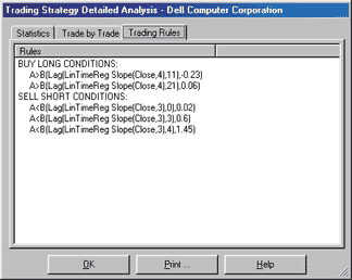
In NeuroShell DayTrader, we loaded a chart of Dell using 30-minute bars. We then inserted a trading strategy with a number of long entry rules, which, in plain English, were, "Buy long when the slope of a line of length x, placed y bars back, exceeds angle z."
The genetic algorithm was instructed to find the proper number of these rules that should be true before a long order is placed, as well as the optimal settings for x, y, and z of each rule. Note it is possible and even desirable for trendlines to overlap.
The genetic algorithm was also given a set of short entry rules, which were optimized with the long entry rules to create a total "reversal" trading strategy optimal for an issue over a given period. The short rules looked for slopes below a particular angle.
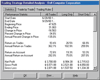
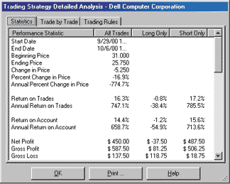
Appropriately, NeuroShell DayTrader is set up to optimize over an earlier in-sample period and then backtest over a later out-of-sample period. We compared both the in-sample optimization period results and the out-of-sample backtest period results with the results from a buy-and-hold strategy. Figure 3 shows the optimal rules found. Figure 4 shows the in-sample period results, and Figure 5 shows the out-of-sample period results.

FIGURE 3: OPTIMAL TRAKING RULES

FIGURE 4: NEUROSHELL IN-SAMPLE PERIOD RESULTS

FIGURE 5: NEUROSHELL OUT-OF-SAMPLE RESULTS
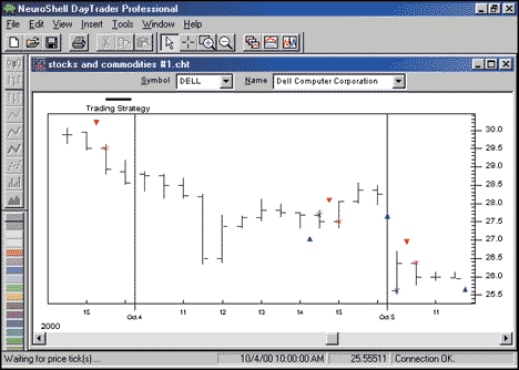
Interestingly, the pattern recognition strategy correctly anticipated the sudden earnings-related drop in Dell between October 4 and 5 and went short on October 4 (Figure 6).

FIGURE 6: NEUROSHELL, PATTERN RECOGNITION STRATEGY
In this trading strategy, we utilized only traditional indicator threshold rules. We did not use a neural network, although we often do feed similar optimized regression slopes into neural networks in NeuroShell DayTrader in order to make trading strategies from neural predictions. We always make use of NeuroShell DayTrader's ability to do "walk forward" out-of-sample testing, giving us a reasonable indication that the model can generalize into the future.
For more variety, we might have also added some under threshold rules to the long entry rule set, and some over threshold rules to the short entry rule set. Another interesting variation on the use of regression slopes is insisting that slope angles not only be over or under thresholds but between thresholds as well.
Finally, you might experiment with restrictions on the ranges of variables. In our example, we accidentally placed severe restrictions on some ranges before optimization, but the genetic algorithm compensated by adjusting other variables.
Users of NeuroShell Trader can go to the STOCKS & COMMODITIES section of the NeuroShell Trader free technical support Website to download the chart in which we built and optimized this strategy. Users of NeuroShell Trader Professional may build similar strategies using daily bars.
--Marge Sherald, Ward Systems Group, Inc. 301 662-7950, sales@wardsystems.com
https://www.neuroshell.com