SYSTEM DESIGN
The Endpoint Fast Fourier Transform System
by Dennis Meyers, Ph.D.
Last time, we explored the Fourier transform, a mathematical technique for analyzing data to determine cyclical component. This time, we use the fast Fourier transform as a trend determinant for a model for trading the Standard & Poor's 500.

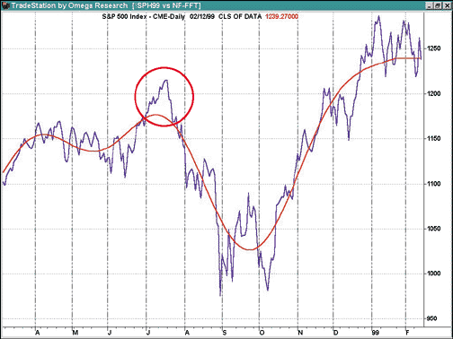
This time, we will demonstrate how to use Fourier transform using the computational algorithm called the fast Fourier transform (FFT) on a walk-forward basis on the S&P 500 continuous futures contract (SP).FIGURE 1: NOISE-FILTERED FFT. Here's the noise-filtered Fft from January 16, 1998, to January 22, 1999. The SP closing high was on July 20, 1998. As can be seen from Figure 1, the FFT curve clearly leads the July 20, 1998, top and is pointing down on that day. This gives the illusion that the FFT curve is a predictive indicator that leads the price series, enabling the market participant to escape the ensuing bear market drop. However, this FFT curve was generated on data from January 16, 1998, to January 22, 1999. What would the FFT curve look like if the curve were generated on July 20, 1998?
THE FFT ILLUSION REVIEW
Figure 1 presents the noise-filtered FFT on the SP from January 16, 1998, to January 22, 1999. The SP closing high was on July 20, 1998. As can be seen from Figure 1, the FFT curve clearly leads the July 20, 1998, top and is pointing down on that day. This gives the illusion that the FFT curve is a predictive indicator that leads the price series, enabling the market participant to escape the ensuing bear market drop. However, this FFT curve was generated on data from January 16, 1998, to January 22, 1999. What would our FFT curve look like if we generated our curve on July 20, 1998?
Figure 2 presents the noise-filtered FFT on the SP from July 15, 1997, to July 20, 1998. As can be seen from the noise-filtered Fft curve generated on July 20, the curve is pointing straight up, giving no indication whatsoever of the coming market drop. Why does this happen? When the FFT went to fit the data, it already knew where all the tops and bottoms were. The FFT mathematics minimize the error between the curve it generates and the real datapoints. This error minimization process forces the generated curve to fit the past data like a glove. As a matter of fact, its almost impossible not to get an excellent fit.
THE ENDPOINT FFT
To avoid the past-data curve-fit illusion, we will create an indicator that walks forward one day at a time. This indicator will calculate the noise-filtered FFT curve but only save the last point, or endpoint, of the curve on the day it is calculated. We will then connect the generated endpoints to produce a curve that matches what we would have seen if we performed the noise-filtered FFT on the endpoint dates.